x2

2

1

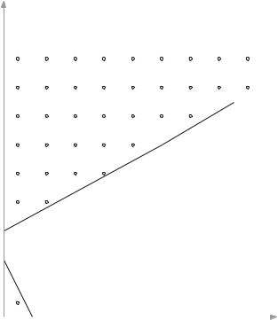
Fig. 2.4 Constraints defining an infeasible LP model

variables. In particular the minimum cost network flow model (with integer flows in and out of the network) and special cases such as the transportation and assignment problems have this property. They will not be discussed further here but references given in Sect. 2.5 discuss them.

2.2 Integer Programming

If all or some of the variables in an, otherwise, LP model are restricted to take integer values then we have a pure or a mixed IP (MIP) model, respectively. As in other branches of mathematics models involving integers are much more difficult to solve than models only involving real numbers. In Sect. 2.4 we discuss the issue of computational complexity and point out that IP models are generally much more difficult to solve than comparably sized LP models.

In Sect. 2.3 we point out that in most practical models the integer variables are restricted to the two values 0 and 1. Hence the connection with the propositional calculus. In this section we confine our attention to solving pure IP models with general integer variables. It will be seen that the methods effectively specialise to

the pure and mixed 0–1 case. For completeness we solve an illustrative model by the decision procedure illustrated in Example 1.9. Then we discuss the more efficient methods employed in practice. We consider the following example.

Example 2.7 Solve the following IP model using the decision procedure for arithmetic without multiplication

·− z + x2 0

·− x2 0)

Since the variable eliminated (x1) has a coefficient of 1 in the equation in (2.46) no congruences are needed in (2.47).

We rewrite this in the form

·4x2 2z + 3

·2(4z − 19) 4x2

·4x2 4z

·0 4x2)

Eliminating x2 reduces the system to

· 4z − 19 + s ≡ 0(mod 2))

In order to satisfy the congruence t = 1. The inequality in (2.51) is then obviously true showing the IP to be feasible.

The maximum value of z satisfying (2.50) is 6 arising from the first inequality in (2.50). This inequality arises from the second and third inequalities in (2.48)

showing that 10 4x2 15 making x2 = 3. These inequalities in turn arise from the equation and third and fourth of the inequalities in (2.47). The (unique) solution is therefore

We now use the above example to illustrate the method usually used in practice for solving IP models. It is usually called the ‘branch-and-bound’ algorithm for reasons which will become apparent.

2.2.1 The Branch-and-Bound Algorithm

Example 2.8 Solve the model in Example 2.7 by the branch-and-bound algorithm.

The first step in this method is to remove the integrality requirements and solve the resultant LP model. This is referred to as the LP relaxation. LP is computationally ‘easy’ compared with IP, as discussed in Sect. 2.5. If the optimal solution to the LP relaxation turns out to be integral then this will also be an optimal solution to the IP. There is an important class of models where this will always be the case. However, for this example, we obtain the fractional solution

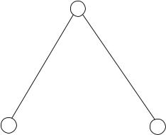
We now choose one of the integer variables (x) whose value has come out fractional (e.g. N + f where N is an integer and 0 < f < 1). There is no loss of generality in stipulating that either x N or x N + 1 since x is not permitted to take any fractional value between N and N + 1. Both these possibilities rule out the current fractional solution. For the example we choose the dichotomy x1 2 or x1 3. The choice of variable x1 over x2 is arbitrary here. In practice it can be made heuristically, i.e. according to plausible (but not guaranteed) rules which might be hoped to produce the optimal integer solution as quickly as possible. For example it might be thought that since x1 is further from its closer integer than x2 this will have more effect than choosing x2. It is convenient to represent this process as a branching in a tree as shown in Fig. 2.5.

At each node we give the solution of the corresponding LP relaxation. Node 2 corresponds to the original model together with the appended constraint x1 2. Node 3 corresponds to the original model together with the appended constraint x1 3. We number the nodes in order of the creation of the corresponding models. Besides the choice of branching variable there is also a choice of order in which to solve the LP relaxations of the nodes created. It is convenient to solve each of the two resultant LP models (the ‘son’ and ‘daughter’) immediately after their creation. It can be seen that the objective values corresponding to the LP relaxations of the two nodes have both got ‘worse’ (declined for a maximisation or increased for a

Fig. 2.5 A branch in the branch-and-bound algorithm

minimisation). This would be expected since extra constraints are being added. In fact they might not change if there were alternate solutions.

At this stage we have a choice of waiting nodes to ‘develop’, i.e. choose which node to branch from. This choice can again be made arbitrarily or heuristically. For example we might choose to develop node 3 in preference to node 1 since its objective has declined less (and there is therefore more chance of a better integer solution down this branch). For our example we continue this process and illustrate it in Fig. 2.6.

At node 5 the LP relaxation (and therefore the corresponding IP) is infeasible. This result is likely to happen as we are adding progressively stronger constraints down a branch. Once a node has become infeasible there is no sense in developing it further. It is said to have been fathomed. Node 4 is then developed in preference to the other waiting node 2 if we use the heuristic that the objective of the LP relaxation at node 4 is better than that at node 2. At node 6 we obtain an integer solution with an objective value of 6. Again there is no sense in developing this node further which is also said to have been fathomed. Since the objective value is better than that at node 2 no better integer solution can be obtained by developing that node. It is also, therefore, said to have been fathomed. The value of the best integer solution found to date provides a bound (hence the use of this word in the title of the method) on the optimal objective value which we have used to terminate the branch at node 2. Solving the LP relaxation at node 7 gives an objective value of 5 12 which again is below the current bound allowing us to terminate this branch. Since there are no more waiting nodes the integer solution found at node 6 has been shown to be optimal. This is the solution already obtained from Example 2.7 and given in (2.53).

Although we have obtained the optimal integer solution there is no guarantee that there might not be other (suboptimal) integer solutions if we had developed nodes 2 and 7. Exercise 2.6.8 involves developing these nodes to see if there are other integer (non-optimal) solutions.

Fig. 2.6 A branch-and-bound tree

Exercise 2.6.9 is to resolve this model by branching on variable x2 instead of x1 at the top of the tree. This will result in a totally different tree but it should be apparent that it must also result in the same optimal objective value and, in this example, the same (unique) optimal solution (although, in general, there could be alternate optimal solutions).

A feature of this method, which should be remarked on, is that immediately after a branch the branching variable takes the value in the added constraint. This will always happen but there is no reason why the variable will not deviate from this value further down the tree, as for example happens at node 4. Once an extra constraint has been imposed at a branch this extra constraint will apply at all branches below the relevant node. For example x1 is greater than or equal to 3 at all nodes from node 3 and below.

If an integer variable is restricted to a finite range of values (as is normally the case in practice) then it should be apparent that this method must converge. In the worse case, the branching process will result in fixing the integer variables at all the (finite number of) possible values at different nodes. This could result in an exponential number of nodes. The potential number of nodes at each successive level doubles giving 2n nodes at level n. Exercise 2.6.10 demonstrates this. However, if some of the integer variables are not restricted to lie in a finite range then there is no guarantee that the method will terminate. Example 2.9 demonstrates this. This shows that branch-and-bound is not formally a decision procedure for IP in contrast to the method illustrated in Example 2.7.

Notice (for example) that the right branch from node 1 (x1 3) and the left branch from node 4 (x1 3) have fixed x1 at 3.

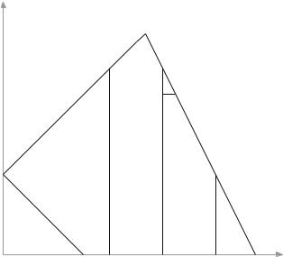
It is useful to illustrate the branch-and-bound method, as performed in Fig. 2.6, geometrically in Fig. 2.7.

C

E H

I J

D

A F G K

Fig. 2.7 A geometrical representation of branch-and-bound

ABCD represents the feasible region of the LP relaxation. The optimal solution of the LP relaxation corresponds to vertex C. By branching on x1 we create the two regions ABEF and GHD corresponding to the LP relaxations at nodes 2 and 3. Vertices E and H correspond to the solutions at those nodes. Branching on x2 at node 3 creates an empty feasible region for x2 4 and the region GIJD for x2 3. The solution at node 4 corresponds to vertex J. Branching on x1 creates the feasible regions GI (one dimensional) and KLD. The solutions at nodes 6 and 7 correspond to vertices I and L. I clearly corresponds to the optimal integer solution.

Example 2.9 Demonstrate that branch-and-bound does not terminate with the following model:

Minimise

x1, x2 Z

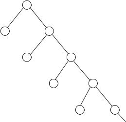
The resulting branch-and-bound tree is given in Fig. 2.8. It should be apparent that the tree will never terminate producing LP relaxations with ever-increasing objective values. Figure 2.9 demonstrates what is happening. The LP relaxation at node 1 corresponds to point A. After branching on x2 we have alternate (all fractional) solutions to the resulting LP relaxation and choose (arbitrarily) that corresponding to point B. Continuing in this manner we produce solutions at points C,D,. . . . The problem is that the IP has no integer solution (it is infeasible). But branch-and-bound cannot detect this as it keeps finding feasible solutions to the LP relaxations. As mentioned before, in practice, this is unlikely to happen since integer variables usually have finite bounds. But it can be the case that branch-and-bound will take an exorbitant amount of time with some models. Exercise 2.6.11 is to solve this model by the decision procedure demonstrated in Example 2.7. This, of course, terminates finitely showing that there is no solution.

Fig. 2.8 A non-terminating branch-and-bound tree

If we apply branch-and-bound to a mixed IP then we only branch on those variables restricted to take integer values. If the integer variables are restricted to take the values 0 or 1 (in both the pure and mixed cases), as is most common, then the branch-and-bound tree becomes simpler. Each branch fixes a variable at 0 or 1 in the next and all subsequent nodes down the branch.