

8.2 NashTP PT Equilibrium Analysis |
173 |
|
1 |
sim. (pl.1) |
|
1 |
1 |
|
|
|
|
|
|
|
|
|
|
|
|
|
|
|
|
|
|
|
|
|
|
|
|
|
|
|
|
|
1 |
1 |
|
|
|
|
|
||||
|
0.9 |
sim. (pl.2) |
|
Θdem=var. ∆dem=0.02 |
|
|
|
|
sim. (pl.1) |
|
Θdem=var. ∆dem=0.02 |
|
|
|
|
|||||||
|
|
analyt. (pl.1) |
|
|
|
|
|
|
|
|
|
sim. (pl.2) |
|
|
|
|
|
|
|
|
||
1,2 obs |
|
Θ2 |
=0.4 ∆2 |
|
|
|
|
|
0.05 |
analyt. (pl.1) |
|
2 |
2 |
|
|
|
|
|
||||
|
|
|
|
|
|
|
|
|
|
|
|
|
|
|||||||||
analyt. (pl.2) |
|
=0.03 |
|
|
|
analyt. (pl.2) |
|
Θdem=0.4 ∆dem=0.03 |
|
|
|
|
||||||||||
Θ |
0.7 |
|
|
|
dem |
dem |
|
|
|
1,2 |
obs |
|
|
|
|
|
|
|
|
|
|
|
|
|
|
|
|
|
|
|
|
|
|
|
|
|
|
|
|
|
|||||
throughputs,observed |
|
|
|
|
|
|
|
|
|
delays,observed∆ |
0.04 |
|
|
|
|
|
|
|
|
|
|
|
|
|
|
|
|
|
|
|
|
|
|
|
|
|
|
|
|
|
|
|
|
|
|
|
0.5 |
|
|
|
|
|
|
|
|
|
|
0.03 |
|
|
|
|
|
|
|
|
|
|
|
|
|
|
|
|
|
|
|
|
|
|
|
|
|
|
|
|
|
|
|
|
|
|
0.3 |
|
|
|
|
|
|
|
|
|
|
0.02 |
|
|
|
|
|
|
|
|
|
|
|
|
|
|
|
|
|
|
|
|
|
|
|
|
|
|
|
|
|
|
|
|
|
|
0.1 |
|
|
|
|
|
|
|
|
|
|
0.01 |
|
|
|
|
|
|
|
|
|
|
|
|
|
|
|
|
ΣΘdem >1 |
|
|
|
|
|
|
|
|
|
ΣΘ |
|
>1 |
|
|
||
|
0 |
|
|
|
|
|
|
|
|
0 |
|
|
|
|
|
dem |
|
|
||||
|
|
|
|
|
|
|
|
|
|
|
|
|
|
|
|
|
|
|
|
|||
|
0.1 |
0.2 |
0.3 |
0.4 |
0.5 |
0.6 |
1 0.7 |
0.8 |
0.9 |
|
0.1 |
0.2 |
0.3 |
0.4 |
0.5 |
0.6 |
1 0.7 |
0.8 |
0.9 |
|||
|
|
|
|
|||||||||||||||||||
|
|
|
throughput demand of player 1, |
Θ |
|
|
|
|
|
throughput demand of player 1, Θ |
|
|
|
|||||||||
|
|
|
|
|
|
|
|
dem |
|
|
|
|
|
|
|
|
|
|
dem |
|
|
|
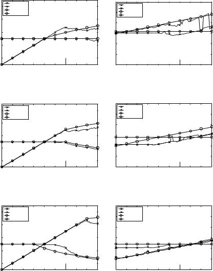
Figure 8.2: Resulting observed QoS parameters of an SSG for two interacting players via
Θ1 , calculated with P, and simulated. Left: observed share of capacity, right: observed
dem 1 2
resource allocation interval. In this figure, ∆dem < ∆dem .
|
|
1 |
sim. (pl.1) |
|
1 |
1 |
|
|
|
|
|
|
sim. (pl.1) |
|
Θ1 |
=var. ∆1 |
=0.02 |
|
|
|
|
||
|
|
|
|
|
|
|
|
|
|
|
|
|
|
|
|||||||||
|
|
0.9 |
sim. (pl.2) |
|
Θdem=var. ∆dem=0.02 |
|
|
|
|
sim. (pl.2) |
|
dem |
dem |
|
|
|
|
|
|||||
|
|
|
analyt. (pl.1) |
|
|
|
|
|
|
|
|
0.05 |
analyt. (pl.1) |
|
2 |
2 |
|
|
|
|
|
||
1,2 |
obs |
analyt. (pl.2) |
|
Θ2 |
=0.4 ∆2 |
=0.02 |
|
|
|
|
analyt. (pl.2) |
|
Θdem=0.4 ∆dem=0.02 |
|
|
|
|
||||||
Θ |
0.7 |
|
|
|
dem |
dem |
|
|
|
1,2 |
obs |
|
|
|
|
|
|
|
|
|
|
||
|
|
|
|
|
|
|
|
|
|
|
|
|
|
|
|
|
|
||||||
throughputs,observed |
|
|
|
|
|
|
|
|
delays,observed∆ |
0.04 |
|
|
|
|
|
|
|
|
|
|
|||
|
|
|
|
|
|
|
|
|
|
|
|
|
|
|
|
|
|
|
|||||
|
|
|
|
|
|
|
|
|
|
|
|
|
|
|
|
|
|
|
|
|
|
|
|
|
|
0.5 |
|
|
|
|
|
|
|
|
|
|
0.03 |
|
|
|
|
|
|
|
|
|
|
|
|
0.3 |
|
|
|
|
|
|
|
|
|
|
0.02 |
|
|
|
|
|
|
|
|
|
|
|
|
|
|
|
|
|
|
|
|
|
|
|
|
|
|
|
|
|
|
|
|
|
|
|
|
|
|
|
|
|
|
|
|
|
|
|
0.01 |
|
|
|
|
|
|
|
|
|
|
|
|
0.1 |
|
|
|
|
|
ΣΘdem >1 |
|
|
|
|
|
|
|
|
|
ΣΘ |
|
>1 |
|
|
|
|
|
0 |
|
|
|
|
|
|
|
|
0 |
|
|
|
|
|
dem |
|
|
||||
|
|
|
|
|
|
|
|
|
|
|
|
|
|
|
|
|
|
|
|
|
|||
|
|
0.1 |
0.2 |
0.3 |
0.4 |
0.5 |
0.6 |
1 0.7 |
0.8 |
0.9 |
|
0.1 |
0.2 |
0.3 |
0.4 |
0.5 |
0.6 |
1 0.7 |
0.8 |
0.9 |
|||
|
|
|
|
|
|||||||||||||||||||
|
|
|
|
throughput demand of player 1, |
Θ |
|
|
|
|
|
throughput demand of player 1, Θ |
|
|
|
|||||||||
|
|
|
|
|
|
|
|
|
dem |
|
|
|
|
|
|
|
|
|
|
dem |
|
|
|
Figure 8.3: Resulting observed QoS parameters of an SSG for two interacting players via
Θ1 , calculated with P, and simulated. Left: observed share of capacity, right: observed
dem 1 2
resource allocation interval. In this figure, ∆dem = ∆dem .
|
|
1 |
sim. (pl.1) |
|
Θ1 |
=var. ∆1 |
|
|
|
|
|
|
sim. (pl.1) |
|
Θdem1 |
=var. ∆dem1 |
=0.02 |
|
|
|
|
||
|
|
0.9 |
|
=0.02 |
|
|
|
|
|
|
|
|
|
||||||||||
|
|
sim. (pl.2) |
|
dem |
dem |
|
|
|
|
|
|
sim. (pl.2) |
|
|
|
|
|
|
|
|
|||
|
|
|
analyt. (pl.1) |
|
|
|
|
|
|
|
|
0.05 |
analyt. (pl.1) |
|
2 |
2 |
|
|
|
|
|
||
1,2 |
obs |
analyt. (pl.2) |
|
2 |
2 |
|
|
|
|
|
|
analyt. (pl.2) |
|
Θdem=0.4 ∆dem=0.01 |
|
|
|
|
|||||
|
|
|
Θdem=0.4 ∆dem=0.01 |
|
1,2 |
obs |
|
|
|
|
|
|
|
|
|
|
|||||||
Θ |
0.7 |
|
|
|
|
|
|
|
|
|
|
|
|
|
|
|
|
|
|
||||
throughputs,observed |
|
|
|
|
|
|
|
|
delays,observed∆ |
0.04 |
|
|
|
|
|
|
|
|
|
|
|||
|
|
|
|
|
|
|
|
|
|
|
|
|
|
|
|
|
|
|
|||||
|
|
|
|
|
|
|
|
|
|
|
|
|
|
|
|
|
|
|
|
|
|
|
|
|
|
0.5 |
|
|
|
|
|
|
|
|
|
|
0.03 |
|
|
|
|
|
|
|
|
|
|
|
|
0.3 |
|
|
|
|
|
|
|
|
|
|
0.02 |
|
|
|
|
|
|
|
|
|
|
|
|
|
|
|
|
|
|
|
|
|
|
|
|
|
|
|
|
|
|
|
|
|
|
|
|
|
|
|
|
|
|
|
|
|
|
|
0.01 |
|
|
|
|
|
|
|
|
|
|
|
|
0.1 |
|
|
|
|
|
ΣΘdem >1 |
|
|
|
|
|
|
|
|
|
ΣΘ |
|
>1 |
|
|
|
|
|
0 |
|
|
|
|
|
|
|
|
0 |
|
|
|
|
|
dem |
|
|
||||
|
|
|
|
|
|
|
|
|
|
|
|
|
|
|
|
|
|
|
|
|
|||
|
|
0.1 |
0.2 |
0.3 |
0.4 |
0.5 |
0.6 |
1 0.7 |
0.8 |
0.9 |
|
0.1 |
0.2 |
0.3 |
0.4 |
0.5 |
0.6 |
1 0.7 |
0.8 |
0.9 |
|||
|
|
|
|
|
|||||||||||||||||||
|
|
|
|
throughput demand of player 1, |
Θ |
|
|
|
|
|
throughput demand of player 1, Θ |
|
|
|
|||||||||
|
|
|
|
|
|
|
|
|
dem |
|
|
|
|
|
|
|
|
|
|
dem |
|
|
|
Figure 8.4: Resulting observed QoS parameters of an SSG for two interacting players via
Θ1 , calculated with P, and simulated. Left: observed share of capacity, right: observed
dem 1 2
resource allocation interval. In this figure, ∆dem > ∆dem .
8.2.1Definition and Objective of the Nash Equilibrium
The Nash equilibrium is defined in the following Definition 8.1.
174 |
|
8. The Superframe as Single Stage Game |
|||||
Definition 8.1 (Osborne and Rubinstein 1994) A Nash equi- |
|||||||
librium of |
actions |
in the Single |
Stage Game is a vector of |
ac- |
|||
tions a*=( ai*,a−i* ) Α, with |
Α =× |
i N |
Αi |
with the property |
|||
that for every player i Ν , the action ai* |
is preferred to any |
||||||
other action ai , |
provided that the opponent takes the ac- |
||||||
tion a−i* , |
that |
means |
( ai*,a−i* ) \i ( ai ,a−i* ) for |
all |
|||
ai Ai , i Ν . Here, a−i denotes a j , |
j ≠i with i, j Ν . |
|
|||||
The Nash equilibrium of actions in the SSG is characterized by the fact that for each player i, the particular action ai* maximizes V i(a)=V i(ai ,a−i* ) in Ai for a given a−i* . When operating in Nash equilibrium, no player can profitably deviate from its choice of action, thus the action taken by any player will remain stable as long as QoS requirements do not change. Given the action of the other players, no player has reason to take an action than the one that leads to the Nash equilibrium, as each player’s action is an optimal, payoff maximizing response to the opponent player’s action. In general, either none, or a unique, or multiple Nash equilibria may exist in a strategic game.
In a course of an MSG, if a Nash equilibrium exists in the SSG, players that adjust their demands rationally in the sense that they attempt to maximize their payoffs, will end up in an action profile that is a Nash equilibrium. If there is no Nash equilibrium in the SSG, then rational players keep adjusting their demands continuously without meeting a stable point of operation. If multiple Nash equilibria exist in the SSG, then it is not clear to which one the players are adjusting their demands throughout the course of an MSG.
8.2.2Existence of the Nash Equilibrium in the SSG of Coexisting CCHCs
The SSG as it was defined in the previous Chapter 7 allows an uncountable number of actions per player. Such a game is referred to as infinite game (Fudenberg 1991). The analytical approximation of Section 8.1 works with a continuum of actions, whereas a simulation is performed with a large finite set of actions. During simulation, the size of the action set was chosen such that sensitivities to the precision of the discrete grid of actions are negligible. Therefore, the existence of a Nash equilibrium is verified by using a theorem that is known from the theory of infinite games, i.e., games that allow an infinite number of actions per player. The theorem uses an attribute of the payoff, which is referred to as quasi-concavity. Quasi-concavity of a payoff is defined in the following Definition 8.2. The Definition 8.3 recalls another necessary attribute, the continuity of the payoff.
8.2 NashTP PT Equilibrium Analysis |
|
|
|
|
|
|
175 |
||
Definition 8.2 |
For any two actions of a player i, |
ai , bi Ai , |
|||||||
and any action of the opponent player -i, |
a−i A−i , if a pay- |
||||||||
off |
V i( ai ,a−i ) |
of |
player i in |
an SSG satisfies |
|||||
min(V i (ai ,a-i ),V i (bi ,a-i )) ≤V i ( α ai +(1 −α ) bi ,a-i ) |
for |
||||||||
any |
vector |
of |
two |
real |
numbers |
α =( α ,α |
2 |
) 2, |
|
with α1,α2 ( 0...1) , then |
|
|
1 |
|
|
||||
the |
payoff is |
said to |
be |
quasi- |
|||||
concave in Ai . |
|
|
|
|
|
|
|
||
From this definition it follows that a payoff is quasi-concave if and only if every
local maximum in Ai is a global maximum in |
Ai . |
||||
Definition 8.3 |
(Debreu 1959:15) Let the payoff V i( a ) be a |
||||
function from |
Α to |
, and consider an action profile repre- |
|||
sented by the point a ' =( ai ',a−i |
') Α. The payoff V i( a ) is |
||||
continuous |
at |
this |
point |
a ' |
if, when a ''→a ' and |
y' =V i( a '), |
y'' =V i( a '') it follows that y''→ y' . The func- |
||||
tion is continuous in Α if it is continuous at every point of Α .
With these two definitions, it is possible to formulate a sufficient condition for the existence of at least one Nash equilibrium in the SSG. The following Theorem 8.1 for the existence of a Nash equilibrium in an infinite game is taken from Fudenberg (1991).
Theorem 8.1 (Fudenberg 1991:34) Consider a strategic game of whose action spaces Ai are nonempty compact convex subsets of an Euclidean space, i Ν ={1, 2} . If all
payoffs |
V i (ai ,a-i ) are continuous in Α and quasi-concave |
||
in Ai , |
there exists |
a pure |
action Nash equilib- |
rium a* =( ai*, a−i* ) in |
Α =× |
Ai , i, −i Ν . |
|
|
|
i Ν |
|
The theorem is for example proven in Debreu (1952). Note that in the SSG competition model mixed actions are not defined, players take pure actions only (see Section 7.2). Nash equilibria can still exist in the SSG if the conditions of this theorem are not satisfied, as these conditions are sufficient but not necessary.
Proposition 8.1 postulates the existence of a Nash equilibrium in the SSG of two coexisting CCHCs. This proposition is proven underneath.
Proposition 8.1 In the Single Stage Game of two coexisting CCHCs exists a Nash equilibrium in Α =×i Ν Ai .
178 |
|
|
|
|
|
|
|
8. The Superframe as Single Stage Game |
||||||||||||||
|
∂Θi |
|
|
|
|
|
|
Θ−i |
|
∆−i |
∆i |
|
|
|
|
|
|
|
||||
|
|
|
|
|
|
|
|
|
|
|
|
|
|
|
||||||||
|
|
|
|
|
|
|
|
|
|
|
|
|
|
|
||||||||
|
obs |
|
|
|
= |
|
|
dem |
dem |
dem |
|
|
|
|
|
|||||||
|
∂Θi |
|
Θdemi →Θ0i |
|
i |
i |
|
|
−i |
|
|
−i |
|
2 |
|
|
|
|||||
|
dem |
|
i |
i |
|
(Θdem ∆dem +Θdem ∆dem ) |
|
|
i |
i |
||||||||||||
|
|
|
|
|||||||||||||||||||
|
|
|
Θdem >Θ0 |
|
|
|
|
|
|
|
|
|
|
|
|
|
|
|
|
Θdem →Θ0 |
||
|
|
|
|
gradient of |
the curve |
|
for larger demand |
|
|
|
|
|
||||||||||
|
|
|
|
|
|
at intersection point Θ0i |
|
|
|
|
|
|
|
|
||||||||
|
|
= |
Θ−i ∆−i |
|
|
|
|
|
|
|
|
|
|
|
|
|
|
|
|
|||
|
|
dem |
|
dem |
|
|
|
|
|
|
|
|
|
|
|
|
|
|
|
|
||
|
|
|
|
∆i |
|
|
|
|
|
|
|
|
|
|
|
|
|
|
|
|
|
|
|
|
|
|
dem |
|
|
|
|
|
|
|
|
|
|
|
|
|
|
|
|
|
|
Therefore, |
|
|
|
|
|
|
|
|
|
|
|
|
|
|
|
|
|
|
|
|
|
|
|
|
|
Θ−i ∆−i |
|
|
|
∂Θi |
|
|
|
|
|
|
|
|
|
|
|
|
|||
|
|
|
|
|
|
|
|
|
|
|
|
|
|
|
|
|
|
|||||
|
|
|
|
dem |
dem |
< 1 = |
|
obs |
|
|
|
|
|
|
|
|
, |
|
||||
|
|
|
|
∆i |
|
|
|
|
∂Θi |
|
|
|
|
i |
|
|
i |
|
|
|
|
|
|
|
|
|
dem |
|
|
|
|
dem |
|
Θ |
dem |
<Θ |
0 |
|
|
|
|
||||
|
|
|
|
|
|
|
|
|
|
|
|
|
||||||||||
|
|
|
|
|
|
|
|
|
|
|
|
|
|
|
|
|
|
|
|
|||
|
|
|
|
|
|
|
|
gradient of the curve |
|
for smaller |
|
|
|
|||||||||
|
|
|
|
|
|
|
|
demand at intersection point Θ0i |
|
|
|
|||||||||||
since it was required that |
0 < Θ0i <1 . It can be concluded that |
|||||||||||||||||||||
Θobsi is a concave function of Θdemi |
for any demand. It can be |
|||||||||||||||||||||
concluded that Θobsi |
is a concave function in |
Ai . |
■ |
|||||||||||||||||||
The Proposition 8.1 implies the existence of at least one Nash equilibrium, which may not be unique. The uniqueness of Nash Equilibria in the SSG is discussed in the next section.
8.2.3Calculation of Nash Equilibria in the SSG of Coexisting CCHCs
A necessary condition for a to be a Nash equilibrium |
a* =(ai*,a−i* ) Αwith |
the property that for every player i Ν , the action ai* |
is preferred to any other |
action ai , is given by |
|
|
|
|
|
|
|
|
|
|
∂ |
|
|
|
|
|
|
|
|
|
|
|
|
|
|
|
|
|
i |
i |
|
|
|
i |
|
∂Θi |
|
|||
a = a* 0 = grad |
( a ) |
i Ν, |
with grad |
= |
|
dem |
, |
|||||
|
V |
|
|
∂ |
|
|||||||
|
|
|
|
|
|
|
|
|
||||
|
|
|
|
|
|
|
|
|
|
|
|
|
|
|
|
|
|
|
|
|
i |
|
|||
|
|
|
|
|
|
|
|
|
∂∆dem |
|
||
that means for every player i Ν , |
|
|
|
|
|
|
|
|
|
|||
0 = grad i U i ( Θreqi |
, ∆reqi , ∆demi ,Θdemi |
, Θdem−i , ∆dem−i |
) i Ν . |
(8.15) |
||||||||
requirement |
demand |
opponent's demand |
|
|
|
|
|
|||||
8.2 NashTP PT Equilibrium Analysis |
179 |
In the SSG, the utilities U i are concave functions in Ai for any player i, therefore Equation (8.15) is a sufficient condition for a Nash equilibrium (Mangold et al. 2001h).
In a game of two players, Equation (8.15) describes a system of four equations with the four unknown variables ∆demi ,Θdemi ,Θdem−i , ∆dem−i , given the requirements per player. In order to achieve differentiability, when calculating a Nash equilibrium, the utility functions have to be considered piecewisely. From Equation (8.15), the resulting vectors of demands in Nash equilibrium can be calculated numerically, if the requirements of all players and the shaping parameters u, v of the utility function are known. In general, the resulting vectors of demands in a Nash equilibrium can be given in closed form as function of all parameters of the game (resulting vectors of demands in a Nash equilibrium are given by the action profile that is selected when playing the Nash equilibrium). Because of the complexity of the general term of the Nash equilibrium, this is not explicitly shown here.
Depending on the profile of requirements, and given the shaping parameters of the utility function, Nash equilibria can be calculated with Equation (8.15). As an example for the calculation, in the following the Nash equilibrium is calculated for one example.
Let
|
Θ1req |
|
Θreq2 |
|
= |
0.4 |
|
0.4 |
|||
|
∆1 |
, |
∆2 |
|
|
0.023 |
|
, |
0.04 |
|
|
|
|
|
|
|
|
|
|
||||
|
req |
|
req |
|
|
|
|
||||
be the matrix of requirements of |
|
the player 1 |
and 2, both players select their |
|
actions out of the sets |
|
|
|
|
ai Ai = |
|
Θ = [ 0...1] |
|
, |
|
∆ = [ 0...0.1] |
|
||
|
|
|
|
|
as defined in Equation (7.8), with i Ν . Equation (8.15) is used to calculate the Nash equilibria with the following set of equations, where the utility functions are shaped as stated in Equation (7.15).
∂ |
|
U1( Θ1req , ∆1req , ∆1dem ,Θ1dem ,Θdem2 , ∆dem2 ) = 0 |
|
∂Θ1dem |
|
||
|
|
||
∂ |
U1( Θ1req , ∆1req , ∆1dem ,Θ1dem ,Θdem2 , ∆dem2 ) = 0 |
||
∂∆1dem |
|||
|
|
||
180 |
|
|
|
8. The Superframe as Single Stage Game |
|
∂ |
|
U 2 ( Θreq2 , ∆req2 , ∆dem2 |
,Θdem2 ,Θ1dem , ∆1dem ) = 0 |
|
∂Θ2 |
|
||
|
|
|
|
|
|
dem |
|
|
|
|
∂ |
U 2 ( Θreq2 , ∆req2 , ∆dem2 |
,Θdem2 ,Θ1dem , ∆1dem ) = 0 |
|
|
∂∆2 |
|||
|
|
|
|
|
|
dem |
|
|
|
This system of differential equations can be solved numerically for any specific requirement profile. With this solution, the resulting demands in Nash equilibrium are
|
1 |
0.42 |
|
, a |
2 |
0.44 |
|
||
a* = a * = |
0.018 |
|
|
* = |
0.032 |
|
|||
|
|
|
|
|
|
|
|
||
and with Equations (7.12)-(7.16), the resulting payoffs in Nash equilibrium are
V( a * ) = (0.817,1.000).
Both |
players achieve a high payoff |
in this example. However, player 1 suffers |
from |
the competition and the |
allocation process, and its payoff is |
V1( a * ) = 0.817 . Therefore, it cannot completely achieve its QoS requirements in Nash equilibrium. It depends on the services the player 1 attempts to support if it is satisfied with this degradation or not. The Nash equilibrium is achieved either through complete knowledge in one SSG or through adjustment in repeated SSGs, when both players play rational. Playing rational means playing the best response action, i.e., attempting to optimize the payoff by taking the action that results in the highest payoff per SSG.
In general, multiple Nash equilibria can exist in the SSG, which may be the case for some QoS requirements the players attempt to support. Depending on the profile of requirements of the players, the Nash equilibrium in the SSG of two coexisting CCHCs is not always unique. A game with multiple Nash equilibria is given for example in games where both players have very high QoS requirements, such as
|
Θ1req |
|
Θreq2 |
|
= |
0.9 |
0.9 |
|
|||
|
∆1 |
, |
∆2 |
|
|
0.4 |
|
, |
0.4 |
. |
|
|
|
|
|
|
|
|
|
||||
|
req |
|
req |
|
|
|
|
||||
In this game, typically Θobsi |
Θreqi for any i, and thus V( a * ) = (0, 0), for a large |
||||||||||
number of action profiles. This is a result of the shape of the utility function used in all games: for any shaping parameter, the utility function is concave, but not strictly concave.

8.3 ParetoTP PT Efficiency Analysis, and Behaviors |
181 |
8.3Pareto17 Efficiency Analysis, and Behaviors
In a SSG, Nash equilibria are stable and predictable points of operation. Players that take rational actions will automatically adjust into a Nash equilibrium, because it has been shown that at least one Nash equilibrium exists in the SSG. If the Nash equilibrium is unique, then the respective action profile can be predicted as point of operation, as a result of rational behavior. However, there may in general exist action profiles in the SSG that can lead to higher payoffs than what is achieved in Nash equilibrium. If such profiles do not exist, the Nash equilibrium is referred to as Pareto efficient, or equivalently, Pareto optimal. If such a profile exists, the Nash equilibrium is not Pareto efficient. In this case, payoffs may be optimized through actions taken by all players. This is discussed in the following.
The Definition 8.4 highlights the concept of Pareto efficiency, which is also referred to as Pareto optimality.
Definition 8.4 |
(Shubik 1981:347) Let the payoff V i( a ) be |
a function from |
Α to , and consider an action profile rep- |
resented by point a =( ai ,a−i ) Α, with i Ν ; Ν being the set of players of a game. The action profile (the point) is said
to be Pareto efficient (or Pareto optimal) if there is no other action profile a ' =( ai ',a−i ') Α such that V i( a ') ≥V i( a ) for all i Ν and V i( a ') >V i( a ) for at least one i Ν .
Definition 8.4 indicates that there can be one or more Pareto efficient action profiles in the SSG. A unique Nash equilibrium in the SSG that is Pareto efficient is a desirable scenario in the sense that in this case there is no other action profile that allows the usage of radio resources more efficiently, i.e., with larger payoffs for all involved players. It depends on the requirements of the players in the CCHC coexistence game if a Nash equilibrium is Pareto efficient. In general, Nash equilibria are less probable to be Pareto efficient in games where all players require more resources than available, i.e., with high offered traffic.
In addition, in case the Nash equilibrium is not Pareto efficient, a Pareto efficient action profile is reached if all players deviate from the Nash equilibrium point. If one player alone deviates, it achieves a lower payoff than before, according to the definition of a Nash equilibrium. Thus, when deviating from action profiles that are Nash equilibria and not Pareto efficient towards action profiles that are not
17 Vilfredo Pareto (1848-1923), Italian economist.