Proof. K is a vector space of dimension 2 over F . Extend {1} to a basis {1, α}

K over F , and K = F (β) where β2 = b + (a2/4) = γ F . Hence K = F (√γ ).

Proposition 11.17. If F is an extension field of R of finite degree, then F is isomorphic to R or C.

Proof. Let [F : R] = n. If n = 1, then F is equal to R. Otherwise, n > 1 and F contains some element α not in R. Now {1, α, α2, . . . , αn} is a linearly dependent set of elements of F over R, because it contains more than n elements; hence there exist real numbers λ0, λ1, . . . , λn, not all zero, such that

λ0 + λ1α + · · · + λnαn = 0.

The element α is therefore algebraic over R so since the only irreducible polynomials over R have degree 1 or 2, α must satisfy a linear or quadratic equation over R. If it satisfies a linear equation, then α R, contrary to our hypothesis. Therefore, [R(α) : R] = 2, and, by Proposition 11.16, R(α) = R(√γ ). In this

Therefore, the field F contains a subfield C = R(α) isomorphic to the complex numbers and [F : C] = [F : R]/2, which is finite. By an argument similar to the above, any element of C is the root of an irreducible polynomial over C. However, the only irreducible polynomials over C are the linear polynomials, and all their roots lie in C. Hence F = C is isomorphic to C.

Example 11.18. [R : Q] is infinite.

√

Solution. The real number n 2 is a root of the polynomial xn − 2, which, by Eisenstein’s criterion, is irreducible over Q. If [R : Q] were finite, we could use Theorem 11.6 and Corollary 11.12 to show that

This is a contradiction, because no finite integer is divisible by every integer n. Hence [R : Q] must be infinite.

GALOIS FIELDS

In this section we investigate the structure of finite fields; these fields are called

´

Galois fields in honor of the mathematician Evariste Galois (1811–1832).

226 11 FIELD EXTENSIONS

We show that the element 1 in any finite field generates a subfield isomorphic to Zp , for some prime p called the characteristic of the field. Hence a finite field is some finite extension of the field Zp and so must contain pm elements, for some integer m.

The characteristic can be defined for any ring, and we give the general definition here, even though we are mainly interested in its application to fields.

For any ring R, define the ring morphism f : Z → R by f (n) = n · 1R where 1R is the identity of R. The kernel of f is an ideal of the principal ideal ring Z; hence Kerf = (q) for some q 0. The generator q 0 of Kerf is called the characteristic of the ring R. If a R then qa = q(1R a) = (q1R )a = 0, Hence if q > 0 the characteristic of R is the least integer q > 0 for which qa = 0, for all a R. If no such number exists, the characteristic of R is zero. For example, the characteristic of Z is 0, and the characteristic of Zn is n.

Proposition 11.19. The characteristic of an integral domain is either zero or prime.

Proof. Let q be the characteristic of an integral domain D. By applying the morphism theorem to f : Z → D, defined by f (1) = 1, we see that

=

But f (Z) is a subring of an integral domain; therefore, it has no zero divisors, and, by Theorem 8.11, q must be zero or prime.

The characteristic of the field Zp is p, while Q, R, and C have zero characteristic.

Proposition 11.20. If the field F has prime characteristic p, then F contains a subfield isomorphic to Zp . If the field F has zero characteristic, then F contains a subfield isomorphic to the rational numbers, Q.

Proof. From the proof of Proposition 11.19 we see that F contains the subring f (Z), which is isomorphic to Zp if F has prime characteristic p. If the characteristic of F is zero, f : Z → f (Z) is an isomorphism. We show that F contains the field of fractions of f (Z) and that this is isomorphic to Q.

Let Q = {xy−1 F |x, y f (Z)}, a subring of F . Define the function

f˜: Q → Q

by f˜(a/b) = f (a) · f (b)−1. Since rational numbers are defined as equivalence classes, we have to check that f˜ is well defined. We can show that f˜(a/b) = f˜(c/d) if a/b = c/d. Furthermore, it can be verified that f˜ is a ring isomorphism. Hence Q is isomorphic to Q.

Lemma 11.24. If g and h are elements of an abelian group of orders a and b, respectively, there exists an element of order lcm(a, b).

by Lemma 4.36. But xy = lcm(a, b) by Theorem 15 of Appendix 2 because xi + yi = max(ai , bi ) for each i.

Lemma 11.25. If the maximum order of the elements of an abelian group G is r, then xr = e for all x G.

Proof. Let g G be an element of maximal order r. If h is an element of order t, there is an element of order lcm(r, t) by Lemma 11.24. Since lcm(r, t) r, t divides r. Therefore, hr = e.

Theorem 11.26. Let GF(q) be the set of nonzero elements in the Galois field GF(q). Then (GF(q) , ·) is a cyclic group of order q − 1.

Proof. Let r be the maximal order of elements of (GF(q) , ·). Then, by

Lemma 11.25,

xr − 1 = 0 for all x GF(q) .

Hence every nonzero element of the Galois field GF(q) is a root of the polynomial xr − 1 and, by Theorem 9.6, a polynomial of degree r can have at most r roots over any field; therefore, r q − 1. But, by Lagrange’s theorem, r|(q − 1); it follows that r = q − 1.

(GF(q) , ·) is therefore a group of order q − 1 containing an element of order q − 1 and hence must be cyclic.

A generator of the cyclic group (GF(q) , ·) is called a primitive element of GF(q). For example, in GF(4) = Z2(α), the multiplicative group of nonzero elements, GF(4) , is a cyclic group of order 3, and both nonidentity elements α and α + 1 are primitive elements.

If α is a primitive element in the Galois field GF(q), where q is the power of a prime p, then GF(q) is the field extension Zp (α) and

GF(q) = {1, α, α2, . . . , αq−2}.

Hence

GF(q) = {0, 1, α, α2, . . . , αq−2}.

Example 11.27. Find all the primitive elements in GF(9) = Z3(α), where α2 + 1 = 0.

Solution. Since x2 + 1 is irreducible over Z3, we have

GF(9) = Z3[x]/(x2 + 1) = {a + bx|a, b Z3}.

The nonzero elements form a cyclic group GF(9) of order 8; hence the multiplicative order of each element is either 1, 2, 4, or 8.

In calculating the powers of each element, we use the relationship α2 = −1 = 2. From Table 11.3, we see that 1 + α, 2 + α, 1 + 2α, and 2 + 2α are the primitive elements of GF(9).

Proposition 11.28.

(i)zq−1 = 1 for all elements z GF(q) .

(ii)zq = z for all elements z GF(q).

(iii)If GF(q) = {α1, α2, . . . , αq }, then zq − z factors over GF(q) as

(z − α1)(z − α2) · · · (z − αq ).

Proof. We have already shown that (i) is implied by Lemma 11.25. Part (ii) follows immediately because 0 is the only element of GF(q) that is not in GF(q) .

For example, in GF(4) = Z2[x]/(x2 + x + 1) = {0, 1, α, α + 1}, and we have

(z + 0)(z + 1)(z + α)(z + α + 1) = (z2 + z)(z2 + z + α2 + α) = (z2 + z)(z2 + z + 1)

= z4 + z = z4 − z.

TABLE 11.3. Nonzero Elements of GF(9)

An irreducible polynomial g(x), of degree m over Zp , is called a primitive polynomial if g(x)|(xk − 1) for k = pm − 1 and for no smaller k.

Proposition 11.29. The irreducible polynomial g(x) Zp [x] is primitive if and only if x is a primitive element in Zp [x]/(g(x)) = GF(pm).

Proof. The following statements are equivalent:

(i)x is a primitive element in GF(pm) = Zp [x]/(g(x)).

(ii)xk = 1 in GF(pm) for k = pm − 1 and for no smaller k.

(iii)xk − 1 ≡ 0 mod g(x) for k = pm − 1 and for no smaller k.

For example, x2 + x + 1 is primitive in Z2[x]. From Example 11.27, we see that x2 + 1 is not primitive in Z3[x]. However, 1 + α and 1 + 2α = 1 − α are primitive elements, and they are roots of the polynomial

(x − 1 − α)(x − 1 + α) = (x − 1)2 − α2 = x2 + x + 2 Z3[x].

Hence x2 + x + 2 is a primitive polynomial in Z3[x]. Also, x2 + 2x + 2 is another primitive polynomial in Z3[x] with roots 2 + α and 2 + 2α = 2 − α.

Example 11.30. Let α be a root of the primitive polynomial x4 + x + 1 Z2[x]. Show how the nonzero elements of GF(16) = Z2(α) can be represented by the powers of α.

Arithmetic in GF(16) can very easily be performed using Table 11.4. Addition is performed by representing elements as polynomials in α of degree less than 4, whereas multiplication is performed using the representation of nonzero elements as powers of α. For example,

= α−6 + α + α2

= α9 + α + α2 since α15 = 1

=α + α3 + α + α2

=α2 + α3.

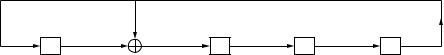
The concept of primitive polynomials is useful in designing feedback shift registers with a long cycle length. Consider the circuit in Figure 11.2, in which the square boxes are delays of one unit of time, and the circle with a cross inside represents a modulo 2 adder.

If the delays are labeled by a representation of the elements of GF(16), a single shift corresponds to multiplying the element of GF(16) by α. Hence, if the contents of the delays are not all zero initially, this shift register will cycle through 15 different states before repeating itself. In general, it is possible to construct a shift register with n delay units that will cycle through 2n − 1 different states before repeating itself. The feedback connections have to be derived from a primitive polynomial of degree n over Z2. Such feedback shift registers are useful in designing error-correcting coders and decoders, random number generators, and radar transmitters. See Chapter 14 of this book and, Lidl and Niederreiter [34, Chap. 6], or Stone [22, Chap. 9].