170 8 RINGS AND FIELDS

It can be verified that these formal power series do form a ring, (R[[x]], +, ·), and that the polynomial ring, R[x], is the subring consisting of those power series with only a finite number of nonzero terms. In fact, the ring of sequences (RN, +, ) is isomorphic to the ring of formal power series (R[[x]], +, ·). The function f : RN → R[[x]] that is defined by f ( a0, a1, a2, · · · ) = a0 + a1x + a2x2 + · · · is clearly a bijection. It follows from the definitions of addition, multiplication, and convolution in these rings, that f is a ring morphism.

FIELD OF FRACTIONS

We can always add, subtract, and multiply elements in any ring, but we cannot always divide. However, if the ring is an integral domain, it is possible to enlarge it so that division by nonzero elements is possible. In other words, we can construct a field containing the given ring as a subring. This is precisely what we did following Example 4.2 when constructing the rational numbers from the integers.

If the original ring did have zero divisors or was noncommutative, it could not possibly be a subring of any field, because fields cannot contain zero divisors or pairs of noncommutative elements.

Theorem 8.25. If R is an integral domain, it is possible to construct a field Q, so that the following hold:

(i) R is isomorphic to a subring, R , of Q.

(ii) Every element of Q can be written as p · q−1 for suitable p, q R .

Q is called the field of fractions of R (or sometimes the field of quotients of R).

We verify that this is an equivalence relation.

(i) (a, b) (a, b), since ab = ba.

(ii) If (a, b) (c, d), then ad = bc. This implies that cb = da and hence that (c, d) (a, b).

(iii)If (a, b) (c, d) and (c, d) (e, f ), then ad = bc and cf = de. This implies that (af − be)d = (ad)f − b(ed) = bcf − bcf = 0. Since R has no zero divisors and d = 0, it follows that af = be and (a, b) (e, f ).

Hence the relation is reflexive, symmetric, and transitive.

Denote the equivalence class containing (a, b) by a/b and the set of equivalence classes by Q. As in Q, define addition and multiplication in Q by

These operations on equivalence classes are defined in terms of particular repre-

sentatives, so it must be checked that they are well defined. If a/b = a /b and c/d = c /d , then ab = a b and cd = c d. Hence

(ad + bc)(b d ) = (ab )dd + bb (cd ) = (a b)dd + bb (c d)

defined.

It can now be verified that (Q, +, ·) is a field. The zero is 0/1, and the identity is 1/1. For example, the distributive laws hold because

=a · c + a · e . b d b f

If we take R = Z to be integers in the above construction, we obtain the rational numbers Q as the field of fractions.

If R is an integral domain, the field of fractions of the polynomial ring R[x] is called the field of rational functions with coefficients in R. Its elements can be considered as fractions of one polynomial over a nonzero polynomial.

A (possibly noncommutative) ring is called a domain if ab = 0 if and only if a = 0 or b = 0. Thus the commutative domains are precisely the integral domains. In 1931, Oystein Ore (1899–1968) extended Theorem 8.25 to a class of domains (now called left Ore domains) for which a ring of left fractions can be constructed that is a skew field (that is, a field that is not necessarily commutative). On the other hand, in 1937, A. I. Mal’cev (1909–1967) discovered an example of a domain that cannot be embedded in any skew field. The simplest example of a noncommutative skew field is the ring of quaternions (see Exercise 8.36). It has infinitely many elements, in agreement with a famous theorem of J. H. M. Wedderburn, proved in 1905, asserting that any finite skew field is necessarily commutative.

CONVOLUTION FRACTIONS

We now present an application of the field of fractions that has important implications in analysis. This example is of a different type than most of the applications in this book. It can be omitted, without loss of continuity, by those readers not interested in analysis or applied mathematics.

We construct the field of fractions of a set of continuous functions, and use it to explain two mathematical techniques that have been used successfully by engineers and physicists for many years, but were at first mistrusted by mathematicians because they did not have a firm mathematical basis. One such technique was introduced by O. Heaviside in 1893 in dealing with electrical circuits; this is called the operational calculus, and it enabled him to solve partial differential equations by manipulating differential operators as if they were algebraic quantities. The second such technique is the use of impulse functions in applied mathematics and mathematical physics. In 1926, when solving problems in relativistic quantum mechanics, P. Dirac introduced his delta function, δ(x), which has the property that

If we use the usual definition of functions, no such object exists. However, it can be pictured in Figure 8.1 as the limit, as k tends to zero, of the functions

δk (x), where

= 1/k δk (x) 0

Each function δk (x) vanishes outside the interval 0 x k and has the prop-

erty that

∞

δk (x) dx = 1.

−∞

w

x

T

t

x

Figure 8.2

putting u = w − t. This integration is over the triangle in Figure 8.2 so, changing the order of integration,

x w

(f (g h))(x) = f (t)g(w − t)h(x − w) dt dw,

00

x

= (f g)(w)h(x − w) dw = ((f g) h)(x).

0

The distributive laws follow because

x

((f + g) h)(x) = (f (t) + g(t))h(x − t) dt

0

x x

= f (t)h(x − t) dt + g(t)h(x − t) dt

0 0

= (f h)(x) + (g h)(x).

There is no function f in C[0, ∞) with this property, although the Dirac delta “function” does have this property. Hence (C[0, ∞), +, ) satisfies all the axioms for a commutative ring except for the existence of an identity under convolution.

Furthermore, there are no zero divisors under convolution; that is, f g = 0 implies that f = 0 or g = 0. This is a hard result in analysis, which is known as Titchmarsh’s theorem. Proofs can be found in Erdelyi [36] or Marchand [37].

However, we can still construct the field of fractions of this algebraic object in exactly the same way as we did in Theorem 8.25. For example, the even integers under addition and multiplication, (2Z, +, ·) is also an algebraic object that satisfies all the axioms for an integral domain except for the fact that multiplication has no identity. The field of fractions of 2Z is the set of rational numbers; every rational number can be written in the form 2r/2s, where 2r, 2s 2Z.

The field of fractions of (C[0, ∞), +, ) is called the field of convolution fractions, and its elements are sometimes called generalized functions, distributions, or operators. Elements of this field are the abstract entities f/g, where f and g are functions. There is a bijection between the set of elements of the form f g/g and the set C[0, ∞). It is possible to interpret other convolution fractions as impulse functions, discontinuous functions, and even differential or integral operators. The Dirac delta function can be defined to be the identity of this field under convolution; therefore, δ = f/f , for any nonzero function f .

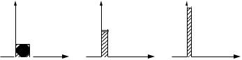
The Heaviside step function illustrated in Figure 8.3 is defined by h(x) = 1 if x 0, and h(x) = 0 if x < 0. The function is continuous when restricted to the nonnegative numbers and, in some sense, is the integral of the Dirac delta function. Convolution by h acts as an integral operator on any continuous function because

x x

(h f )(x) = (f h)(x) = f (t)h(x − t) dt = f (t) dt.

0 0

Hence h f is the integral of f . We can use this to define integration of any generalized function. Take the integral of the convolution fraction f/g to be the fraction (h f )/g.

Denote the inverse of the Heaviside step function by s, so that s = h/ h h. This element s is not a genuine function, but only a convolution fraction. Convolution by s acts, in some sense, as a differential operator in the field of convolution fractions. It is not exactly the usual differential operator, because convolution by s and by h must commute, and s h = h s must be the identity. If f (x) is a continuous function, we know from the calculus, that the derivative of0x f (t) dt is just f (x); however, 0x f (t) dt is not just f (x) but is f (x) − f (0). In fact, if the function f has a derivative,

(s f )(x) = f (x) + f (0)δ(x)

where δ(x) is the identity in the field of convolution fractions. Now, when we calculate h s f , which is equivalent to integrating s f from 0 to x, we obtain the function f back again.

By repeated convolution with s or h, a generalized function can be differentiated or integrated any number of times, the result being another generalized function. We can even differentiate or integrate a fractional number of times. These

h

x

Figure 8.3. Heaviside step function.