Waves_in_Metamaterials

3.1Introduction

Plasmas is an old and respectable subject. It was started by Langmuir1 in the 1920s. Its properties have been studied ever since but not always with the same vigour. Topics rose in response to new applications, and declined on reaching saturation or realizing that the chances of the envisaged solution are fast receding. The development of radio broadcasting led to the discovery of the Earth’s ionosphere that reflects radio waves and is responsible for reception of radio signals when the transmitter is over the horizon. Hannes Alfven’s theory of magnetohydrodynamics (1940) that treated plasma as a conducting fluid has been employed to investigate sunspots, solar flares, the solar wind, star formation and other topics in astrophysics. The interest in thermonuclear fusion came in the wake of the hydrogen bomb. At one time it was believed that fusion, assisted by plasmas, is round the corner. The belief turned out to be not well founded. Later, the invention of lasers opened the new chapter of laser plasma physics with some promise of fusion but that has not been realized either. High-energy physicists hope to use plasma acceleration techniques to dramatically reduce the size and cost of particle accelerators. Among the applications that have come o are microscopy and sensing (see, e.g., Yeatman 1996; Homola 2003; Barnes 2006).

We have enumerated only a fraction of plasma phenomena that could be discussed. The subject is not only old and respectable: it is also very big. Our interest is limited to plasmas on surfaces, the kind that was presented very briefly in Section 1.10. They are important for metamaterial applications that belong to two categories. One is their role in the subwavelength manipulation of images. If μr = 1 and εr = −1 then the plasma resonances will limit the range of spatial frequencies for which the transfer function is approximately flat. This was already briefly discussed in Section 2.12.4. The second relationship with metamaterials is via elements that may exhibit plasma resonances at high enough frequencies. They are mainly nanosized rods and rings and their combinations, reminiscent of electric dipole and loop antennas operating at radio frequencies.

There is, however, a third category that hardly exists at the moment. Nanoscale geometry, for example, allows us to change plasma properties and understanding of this mechanism would allow us to design metamaterial elements with tailored properties. This is just one example that may or may not turn out to be feasible but there are many others. We

3.3Surface plasmon–polaritons. Semi-infinite case,

3.4Surface plasmon–polaritons on a slab: TM polarization 92

3.5Metal–dielectric–metal

3.7 SPP for arbitrary ε and μ 106

1A transparent liquid that remains when blood is cleared of various corpuscles was named plasma (after the Greek word that means ‘formed, jelly-like’) by a Czech medical scientist Purkinje. The Nobel prize-winning American chemist Irving Langmuir first used this term to describe an ionized gas in 1927: Langmuir was reminded of the way blood plasma carries red and white corpuscles by the way an electrified fluid carries electrons and ions. This analogy is, however, slightly odd: blood plasma is blood that is free from blood corpuscles; electric plasma would lose its properties if we were to get rid of free charges in it.

2If we plot a dispersion curve and we find that the frequency is independent of the wave number then it is tempting to call it a non-dispersive wave—and some authors indeed do that. On the other hand, if we remember the original aim of the dispersion curves to show the change of wave velocity with frequency then it is quite obvious that a horizontal line is very dispersive. The phase velocity ω/k varies strongly as a function of k. The only dispersionless curve is a straight line that goes through the origin.

3Admittedly classical physics fails when the propagation length of the mode and the wavelength are comparable with atomic distances (Yang et al., 1991) but we are very far from that limit.

ω, being a constant independent of k, means that only a single value of the frequency, the plasma frequency, is allowed, while the wave number can be arbitrary. Does this equation, which gives a straight horizontal line on an ω–k diagram, show a dispersive behaviour? The answer is yes.2 Of course not all charged-particle systems show such behaviour. An ionic crystal, e.g. sodium chloride, is made up of positively and negatively charged Na+ and Cl− ions. The ions are so tightly bound to one another by electrostatic forces that they cannot move about freely; this system supports acoustic rather than plasma waves. And yet both plasma waves and acoustic waves show remarkable similarities in their ability to interact with electromagnetic waves, giving rise to hybrid modes. And that brings us to the point where we have to say something about terminology. As an electromagnetic wave propagates through a polarizable medium, the polarization it induces modifies the wave and the electromagnetic wave becomes coupled to the induced polarization. We could call this a hybrid mode because its properties depend both on those of the electromagnetic wave and also of the medium. The problem is then that apart from vacuum we nearly always have hybrid modes because the properties of the medium can very rarely be completely disregarded. The argument may then be used that we call them hybrid modes only when the e ect of the medium is significant. This is apparently what happened to acoustic and plasma waves. When they significantly alter the properties of electromagnetic waves they acquire the postfix ‘polariton’. And if that does not sound su ciently pretentious their name is also upgraded. They change from the classical3 ‘plasma waves’ and ‘acoustic waves’ to ‘plasmons’ and ‘phonons’ ending up eventually as plasmon–polaritons and phonon–polaritons. To make things even more complicated we shall have to distinguish between bulk plasmon–polaritons that propagate inside a homogeneous medium, and surface plasmon–polaritons that stick to a surface. Most physicists refer to them nowadays by the acronym SPP.

We shall first look at bulk plasmon–polaritons in Section 3.2 on the basis of the Drude model, and then find the conditions for the existence

4Taking, for instance, the electron density in a typical metal as Ne = 6 ×1028 m−3 we can calculate that ωp = 2π × 2.2×1015 s−1, which corresponds to the wavelength λp = 2πc/ωp = 136 nm, which lies in the ultraviolet.

78 Plasmon–polaritons

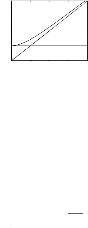
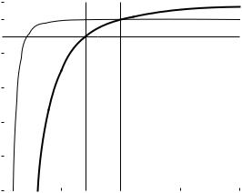
Fig. 3.1 Dispersion of bulk plasmon– polaritons, of plasmons and of the electromagnetic wave in vacuum

5There is a stop band for ω < ωp. Note a general feature (Tilley, 1988) that surface modes can be found within the bulk mode stop bands. It is in this range that our other type of plasmon– polariton, the SPP, can propagate.

It is plotted in Fig. 3.1 as a function of k/kp (where kp = ωp/c), together with the ‘light line’ k = ω/c of the electromagnetic wave in vacuum and with the horizontal dispersion line ω = ωp.

The dispersion curve in Fig. 3.1 may be seen as resulting from the crossing of the bulk plasmon line ω = ωp and the light line k = ω/c. A possible way of interpreting the dispersion equation (3.6) is that there is no longer a pure electromagnetic and a pure plasma wave. Instead, the plasma wave interacts strongly with light, resulting in our bulk plasmon– polariton. The asymptotic and limiting cases for the dispersion are

At high frequencies the bulk mode lies close to the light line and is lightlike; at low wave numbers it moves away from the light line until the cut- o plasma frequency is reached. Bulk plasmon–polaritons of frequency below the plasma frequency cannot propagate5 in plasma because its free electrons screen the electric field of the light. Bulk plasmon–polaritons of frequency above the plasma frequency can propagate through plasma because the electrons cannot respond fast enough to screen it.

Since many of the properties of plasmon–polaritons are similar to those of phonon–polaritons it may be worthwhile to include here a brief note on the latter. The interaction is then between the electromagnetic wave and the optical branch (optical phonons) of the acoustic wave in an ionic crystal. There, the dielectric function has a form

6Note that ε0 in eqn (3.8) is not the free-space permittivity but the value of the dielectric constant at ω = 0.

with ωT the so-called TO (transverse optical) phonon frequency and ωL = ωT ε0/ε∞ the LO (longitudinal optical) phonon frequency (see, e.g., Kittel 1963).6 The asymptotic and limiting cases here are

3.3Surface plasmon–polaritons. Semi-infinite case, TM polarization

The electromagnetic field of SPPs at a dielectric–metal interface is obtained from the solution of Maxwell’s equations in each medium, and the associated boundary conditions. The latter express the continuity of the tangential components of the electric and magnetic fields across the interface. A further obvious condition is that the fields must decline away from the boundary and vanish infinitely far away.

3.3.1Dispersion. Surface plasmon wavelength

We consider now a plane interface z = 0 between two semi-infinite media, the first one being vacuum, air or a dielectric with the permittivity, ε1, taken here as frequency-independent; the second one being a metal with the permittivity, ε2, described by the Drude model (eqn (3.2)). We shall first look at the case of TM polarization. Recalling the results from Section 1.10 the conditions for the existence of a surface mode propagating along the surface in the x direction8 are given as

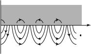
The first of these conditions, requiring that the dielectric constant is changing sign at the boundary, has a simple meaning (Barnes, 2006). A surface mode involves charges accumulated at the boundary between the metal and the dielectric. The corresponding electric field that is built up would originate on positive charges and terminate on negative charges and do so, in fact, in both medium 1 and medium 2. This is shown schematically in Fig. 3.2. That means that in the presence of surface charges the components of the electric field normal to the surface must have opposite signs.

A boundary condition for the normal component of the displacement field is9

z

Metal E

H

Dielectric

Fig. 3.2 SPP mode. A sketch of charge and electric-field distributions at the metal–dielectric boundary

8 For εr1 + εr2 < 0, μr1 = μr2 = 1 a TM surface mode with components Ex , Ez and Hy and propagating in the x direction is the only option. Explicit calculations show that there is no propagation for this mode in the y direction, nor is there a surface TE mode carrying Hx , Hz and Ey components.

9We have just described the role of surface charges and yet, when it comes to the boundary conditions, we ignore the surface charge. This apparent contradiction is resolved in Appendix D.

80 Plasmon–polaritons

10The positive sign in eqn (3.15) also has physical meaning and yields the Brewster wave discussed in Appendix E.

which is another way of saying that for a surface mode to exist dielectric constants in the two media must have di erent signs. The second condition of eqn (3.10) follows from eqn (1.73), which is given below

It ensures that kx is real so that the mode can propagate along the surface. It is a rather innocent-looking equation but it contains a large amount of information about the properties of SPPs at a single interface. Since εr2 is a function of frequency, eqn (3.12) is the dispersion equation, i.e. it provides the relationship between the frequency and the wave number. Inserting eqn (3.2) from the lossless Drude model into eqn (3.12) we find

Equation (3.13) may then be solved for k0 to obtain the dispersion equation in terms of ω. It looks rather complicated so we shall give here the solution only for εr1 = 1

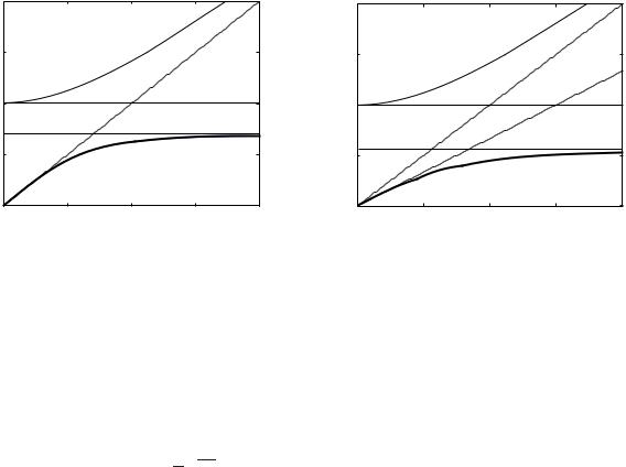
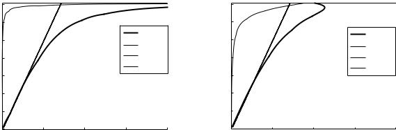
which is not too long. Taking the negative sign10 we shall plot in Figs. 3.3(a) and (b) the dispersion curves at an interface metal–vacuum (εr1 = 1) and metal–glass (εr1 = 2.25).

The dispersion curve shows that at low frequencies the surface mode lies close to the light line and is light-like. As frequency increases, the mode moves away from the light line, gradually approaching an asymptotic limit. This occurs when the permittivities in the two media are of the same magnitude but opposite sign, thus producing a pole in the

is the upper cuto frequency for the surface mode. For vacuum it is

Medium 2 with negative permittivity is often called the surface-active medium, while medium 1 with positive permittivity is called the surfacepassive medium. The reason is quite simple. The terms express the fact

82 Plasmon–polaritons

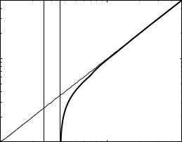
Fig. 3.4 Dispersion curve for the metal–vacuum interface

11A technique often used (see, e.g., Gray and Kupka 2003).

than the free-space wavelength. It would be desirable at this stage to abandon the normalized quantities ω/ωp and k/kp and find the actual values of the various characteristics of the waves, starting with the plasma frequency. For silver, the value of the plasma frequency was determined experimentally by McAlister and Stern (1963) from the dip in the transmission of electromagnetic waves through a thin film. They measured the plasma frequency in terms of electron volt units, giving a value of 3.8 eV, which in SI units corresponds to 918 THz or a wavelength of 326 nm. According to Pendry (2000) the plasma frequency is approximately 9 eV, corresponding to 2183 THz, a big di erence. The main problem is of course that the Drude model, assumed so far is not valid for frequencies close to the plasma frequency. When ω = ωp the dielectric constant is not equal to 1 but to a value of ε0 (a horrendous deviation from the meaning of ε0 in the SI system) due to interband transitions. If we follow Pendry and take its value as 5.7 then εr is equal to −1 at a wavelength of 359 nm. When coming to imaging by a silver lens then this is the wavelength range at which successful imaging was obtained (see, e.g., Melville and Blaikie 2005). Can we save the Drude model without contradicting experimental results? We can do it by choosing the plasma frequency so that the Drude relation remains approximately true11 in the critical region around εr = −1. This choice led us to fp = 1200 THz. We can now plot (Fig. 3.4) the wavelength of the SPP mode λSPP = 2π/kx versus free-space wavelength λ = 2πc/ω. As the free space wavelength approaches the asymptotic value λs = 2πc/ωs the SPP wavelength becomes much shorter than the free-space wavelength, opening up the possibility for subwavelength manipulation of the fields. For larger values of the free-space wavelength, λSPP is only marginally smaller than λ.

In view of the dispersion equations derived we should say here a few more words about terminology. The logical thing would be to call the waves surface plasmon–polaritons for small kx when the dispersion curve is close to that of electromagnetic waves in free space and it is some kind

permittivity H’, − H"

3.3Surface plasmon–polaritons. Semi-infinite case, TM polarization 83

kx/kp

(a)

kx/kp

(b)