

Waves_in_Metamaterials
.pdf
|
|
z |
|
H |
x |
t |
H |
|
|
|
w |
3.6 One-dimensional confinement: shells and stripes 105
 y
y
|
|
|
|
|
|
(a) |
|
3.6 |
|
|
|
|
|
|
3.2 |
|
|
|
|
|
0 |
2.8 |
|
|
|
|
|
EE |
|
|
|
|
|
|
|
|
|
|
|
|
|
|
2.4 |
|
aa2b |
|
sa1b ab |
|
|
2 |
sb |
|
|
|
|
|
0 |
0 |
ss1 |
as2 |
|
|
|
ssb |
asb |
b |
b |
|
|
|
0 |
|
|
0.04 |
0.08 |
0.12 |
Thickness t (Pm)
(b)
|
|
|
10 0 |
|
|
|
|
|
|
|
|
10 –1 |
sa0b , aa0b |
|
|
|
|
|
|
|
|
|
|
|
|
|
|
|
|
|
aa2b,sa1b , ab |
|
|
|
|
sa0 , aa0 |
0 |
–2 |
|
|
|
|
|
|
DE |
|
|
|
|
|
|||
b |
b |
10 |
|
|
|
|
|
|
|
|
|
|
|
|
|||
|
|
|
|
ss0b |
sb |
|
|
|
|
|
|
10 –3 |
|
|
|
|
|
|
|
|
10 –4 |
sb as0b ss1b asb2 |
|
|
|
|
0.16 |
0.2 |
|
0.04 |
0.08 |
0.12 |
0.16 |
0 2 |
|
|
0 |
|||||||
Thickness t (Pm)
(c)
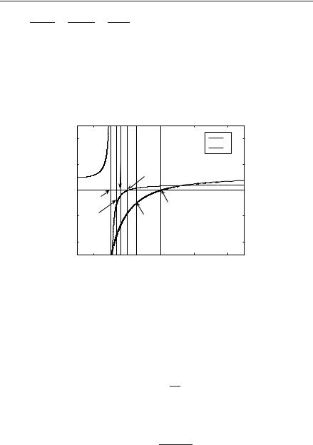
Fig. 3.28 Metallic stripe. (a) Sketch of the geometry. (b), (c) Dispersion with thickness of the first six modes. Also shown the ab and sb modes for w → ∞ for comparision. From Berini (2000b). Copyright c 2000 by the American Physical Society
which they cannot propagate and some of the modes also have a cuto thickness.
For a stripe width of w = 0.5 μm the normalized propagation and attenuation coe cients are plotted in Figs. 3.28(b) and (c) for the first six modes as a function of stripe thickness. The sb and ab modes of the 2D structure are also shown for comparison. As may be expected, the antisymmetric modes have higher attenuation than the symmetric modes. The most relevant conclusion is that the 1D stripe geometry is in no way worse than the amply analyzed 2D geometry. In fact, it may be much better, at least in theory. The attenuation of two of the higher modes may be seen to decrease rapidly before they reach cuto . Presumably, it happens at the expense of confinement. The ss0b mode has probably more practical significance. If we compare it with the sb mode at the lowest thicknesses shown, below 20 nm, we find that the attenuation of the stripe mode is very considerably below that of the 2D planar mode, and the attenuation can be further reduced by decreasing the stripe width.
Stripes having di erent dielectrics for substrates and superstrates have also been investigated by Berini (2001). Small di erences in the upper and lower dielectric constants have been found to lead to larger di erences in propagation properties. There has been no reply given as yet to

106 Plasmon–polaritons
the question posed by the very large propagation lengths (see Fig. 3.25) obtained theoretically by Wendler and Haupt (1986), whether they can be realized in stripe form.
18The analogy is not very good because there are no magnetic charges.
3.7SPP for arbitrary ε and μ
Looking at the surface modes at interfaces of two media we have so far assumed that one of the media is a dielectric with μ = 1 and ε being positive and frequency-independent and that the other one is a metal.
The condition of existence of a surface TM mode at a single metal– dielectric interface was given as
εr2/εr1 < −1 , |
(3.52) |
which, assuming the Drude model for a metal, is satisfied below the surface plasma frequency,
ω < |
√ |
ωp |
. |
(3.53) |
|
||||
|
|
1 + εr1 |
|
|
In the case of a metal slab, the SPP modes excited at the two surfaces interact, the dispersion splits into two, one below and another one above the unperturbed dispersion curve. The resulting condition for the existence of surface modes is much more relaxed. In the limit of an infinitely thin slab it is
εr2/εr1 < 0, |
(3.54) |
meaning that |
|
sign(εr2) = sign(εr1) , |
(3.55) |
and the upper SPP branch can reach up to the bulk plasma frequency
ω < ωp . |
(3.56) |
3.7.1SPP dispersion equation for a single interface
We will now generalize these results to the case when ε and μ can take arbitrary values. At this stage we are not concerned with the question of how or whether these values can be realized. For an early treatment see Ruppin (2000). The derivations to follow are based on the work of Darmanyan et al. (2003). The mathematical problems of solving the field equations subject to the boundary conditions are not particularly di cult. There is, however, a problem with terminology. Allowing now the possibility of negative permeability what should we call them? Some people talk about magnetic plasmons,18 which gives the opportunity to call them electric and magnetic surface plasmon–polaritons but that is quite a mouthful and it is unlikely that it would catch on. So we just decided to stick to the original name and in spite of the changes in permeability we shall still call them surface plasmon–polaritons.

3.7 SPP for arbitrary ε and μ 107
Having done the derivation for the case when the permittivity could take negative values it is an easy task to derive the dispersion equations for the surface waves in the general case. The approach is the same. The results are though more far reaching and will have significant implications for the imaging mechanism of the ‘perfect’ lens to be discussed in Chapter 5.
We disregard losses for simplicity. They can be included later if needed. Looking for surface-wave solutions declining exponentially we require the z components of the k vector to be purely imaginary so that both
κ1 |
= |
kx2 |
− εr1μr1k02 |
(3.57) |
|
and |
|
|
|
|
|
|
|
|
|
||
κ2 |
= |
kx2 |
− εr2μr2k02 |
(3.58) |
|
are to be positive and real. The dispersion equation is formally the same as in the case of a metal. It may be obtained from the poles of the field solutions. For the TM polarization it is
|
ζe + 1 = 0 |
(TM case) |
(3.59) |
||||
or |
|
|
|
|
|
|
|
|
κ2 |
|
εr1 |
|
= −1 |
(TM case) , |
(3.60) |
|
κ1 |
εr2 |
|||||
whereas for the TE polarization we obtain |
|
||||||
|
ζm + 1 = 0 |
(TE case) |
(3.61) |
||||
or |
|
|
|
|
|
|
|
|
κ1 |
|
μr2 |
= −1 |
(TE case) . |
(3.62) |
|
|
κ2 |
μr1 |
|||||
Inserting eqns (3.57) and (3.58) into eqn (3.60) we obtain for the TM case
(kx2 − εr2μr2k02)εr12 = (kx2 − εr1μr1k02)εr22 |
(TM case) , |
(3.63) |
|||||
leading to the dispersion equation |
|
|
|||||
k2 |
= k2 |
εr1εr2 |
|
μr1εr2 |
− μr2εr1 |
(TM case) . |
(3.64) |
|
|
εr2 |
− εr1 |
||||
x |
0 εr1 + εr2 |
|
|
|
|||
Similarly for the TE case, inserting eqns (3.57) and (3.58) into eqn (3.62) we obtain the dispersion equation
k2 |
= k2 |
μr1μr2 |
|
εr1μr2 |
− εr2μr1 |
(TE case) . |
(3.65) |
|
|
μr2 |
− μr1 |
||||
x |
0 μr1 + μr2 |
|
|
|
|||

108 Plasmon–polaritons
For the z components of the k vector in the TM case we obtain by using eqns (3.57), (3.58) and (3.64)
κ2 |
= k2 |
ε2 |
εr1εr2 |
|
μr1εr1 |
− μr2εr2 |
(TM case) |
|
|
εr22 |
− εr12 |
||||
1 |
0 |
r1 εr1 + εr2 |
|
|
|||
and |
|
|
|
|
|
|
|
|
|
|
κ22 = κ12ε2 |
(TM case), |
|||
and in the TE case by using eqns (3.57), (3.58) and (3.65)
κ2 |
= k2 |
μ2 |
μr1μr2 |
|
εr1μr1 |
− εr2μr2 |
(TE case) |
|
|
μr22 |
− μr12 |
||||
1 |
0 |
r1 μr1 + μr2 |
|
|
|||
and |
|
|
|
|
|
|
|
|
|
|
κ22 = κ12μ2 |
(TE case) , |
|||
where ε = εr2/εr1 and μ = μr2/μr1.
(3.66)
(3.67)
(3.68)
(3.69)
3.7.2Domains of existence of SPPs for a single interface
It follows immediately from eqn (3.60) that, as both κ1 and κ2 are to be real and positive, for TM modes to exist the condition
εr2εr1 < 0 |
(TM case) |
(3.70) |
must be satisfied. For TE modes, as follows from eqn (3.62) the condition is
μr2μr1 < 0 |
(TE case) . |
(3.71) |
The result for the TM polarization makes good sense. We are talking here about the electric field with its Ez component changing sign across the boundary, a condition compatible with accumulation of charges at the surface, as we discussed earlier for metals. It is important to note that this condition holds for any value of μ: surface TM modes exist only if ε changes sign at the boundary.
The same argument could be applied for the TE polarization, but it is somewhat di cult to provide a simple physical interpretation of the requirement that μ1 and μ2 must be of di erent sign for a TE surface mode to exist. The reason why it is di cult to picture what is going on is that in the case of negative permeability we cannot appeal to our common-sense expectations. Negative-ε materials have received much more attention in the past and the condition εr1εr2 < 0 for the existence of TM surface modes has been known ever since Fano’s article over sixty years ago. It is quite di erent with negative-μ materials. All such materials, constructed so far, have negative permeability within a frequency

3.7 SPP for arbitrary ε and μ 109
band and not below a certain frequency, as it happens with negativepermittivity materials. Also, we cannot think of surface charges. Instead we must consider surface currents, a less familiar concept, and it is particularly di cult to think about it when the structure is discrete.
Returning to the dispersion equations and taking into account that for TM polarization εr2 < 0, eqns (3.64) and (3.66) can be rewritten as
k2 |
= k2 |
εr1μr1 |
|ε|(|ε| + μ) |
(TM case) |
(3.72) |
||||
x |
|
0 |
|
|
|
ε2 − 1 |
|
|
|
and |
|
|
|
|
|
|
|
|
|
κ2 |
= k2 |
εr1μr1 |
1 + |ε|μ |
(TM case) . |
(3.73) |
||||
ε2 − 1 |
|||||||||
|
1 |
|
0 |
|
|
|
|
||
Similarly, taking into account that for TE polarization μr2 < 0, eqns (3.65) and (3.67) can be rewritten as
|
k2 = k2εr1μr1 |
|μ|(|μ| + ε) |
|
(TE case) |
(3.74) |
||||||
|
|
μ2 − 1 |
|||||||||
and |
x |
0 |
|
|
|
|
|||||
|
|
|
|
|
|
|
|
|
|
|
|
|
κ2 = k2εr1μr1 |
1 + |μ|ε |
|
|
|
(TE case) . |
(3.75) |
||||
|
μ2 − 1 |
||||||||||
|
1 |
0 |
|
|
|
|
|||||
The TM and TE surface modes of eqns (3.72) and (3.74) exist if k2 |
, κ2 |
||||||||||
and κ2 |
|
|
|
|
|
|
|
|
|
x |
1 |
are real and positive. In the case of TM polarization, it follows |
|||||||||||
2 |
|
|
|
|
|
|
|
|
|
|
|
from eqn (3.73) that κ12 is positive if either |
|
|
|
||||||||
|
|
|
1 |
|
|
|
|
||||
|
|ε| > 1 |
and |
|
μ > − |
|
|
(TM case) |
(3.76) |
|||
or |
|
|ε| |
|||||||||
|
|
1 |
|
|
|
|
|
|
|||
|
|
|
|
|
|
|
|
|
|||
|
|ε| < 1 |
and |
μ < − |
|
|
(TM case) . |
(3.77) |
||||
|
|ε| |
||||||||||
Similarly, for TE polarization, the condition κ21 > 0 in eqn (3.75) is fulfilled if either
|
|μ| > 1 |
and |
ε > − |
1 |
(TE case) |
(3.78) |
|||
|
|
||||||||
or |
|μ| |
||||||||
|
|
|
|
|
|
|
|
|
|
|
|
|
|
1 |
|
|
|
|
|
|
|μ| < 1 |
and |
|
ε < − |
|
|
|
(TE case). |
(3.79) |
|
|
|μ| |
|
||||||
If κ2 |
is positive then κ2 |
is positive as well, see eqns (3.67) and (3.69). |
|||||||
1 |
|
2 |
|
|
|
|
|
|
|
Similar considerations for the positiveness of kx2 (eqns (3.64) and (3.74)), do not provide any further constraints for the existence of the surface modes. The domains of existence of the TM mode and of the TE mode are plotted in Fig. 3.29 in the plane (ε, μ).
The horizontal dashed line μ = 1 corresponds to the case of the second medium being a metal with a TM surface mode for ε < −1 (εr2 < −εr1) being the only possibility.

110 Plasmon–polaritons
Fig. 3.29 Domains of TM and TE modes for an interface dielectric– metamaterial with arbitrary values of permittivity and permeability
|
6 |
|
|
|
|
|
|
|
4 |
|
|
|
|
|
|
|
|
TM |
|
|
|
|
|
|
2 |
|
|
|
|
μ=1 |
|
1 |
|
|
|
|
|
|
|
|
|
|
|
|
|
|
|
/μ |
|
|
|
|
|
|
|
2 |
0 |
|
|
|
|
|
|
μ=μ |
TE |
|
|
|
|
|
|
|
|
|
|
|
|
||
|
|
|
|
|
|
|
|
|
−2 |
|
|
|
|
|
|
|
−4 |
|
|
|
TE |
|
|
|
−6 |
|
|
TM |
|
|
|
|
−4 |
−2 |
0 |
2 |
4 |
6 |
|
|
−6 |
||||||
|
|
|
|
ε=ε2/ε1 |
|
|
|
It is worth mentioning that there can be no surface modes at the boundary of two left-handed media with εr1, εr2, μr1, μr2 all being negative (Darmanyan et al., 2003) (this corresponds to the first quadrangle of the plane ε, μ).
It is important to note that if, in a certain frequency range, in medium 2 both εr2 and μr2 are negative, i.e. if medium 2 is a left-handed one then a transverse electromagnetic (bulk) wave can propagate with the
dispersion equation |
|
k = ωc √εr2μr2 . |
(3.80) |
For a surface mode (with fields exponentially decaying away from the interface) to exist, its wave vector must be larger than those of the bulk modes in either media, resulting in the condition
kx > max k0 = |
ω |
√ |
|
, k = |
ω |
√ |
|
. |
(3.81) |
|
εr1μr1 |
|
εr2μr2 |
||||||
c |
c |
This is a new feature that we have not met in the case of a metal where surface modes were only found in the stop bands of the bulk modes. In the case of a left-handed metamaterial with both ε2 and μ2 being negative a bulk and a surface mode can coexist at the same frequency. If their dispersion curves ω(k) intersect, only those parts of the surface mode solutions that lie to the right of the bulk modes are meaningful.
3.7.3SPP at a single interface to a metamaterial: various scenarios
The results of the previous section are general and can be used to look at possible SPP modes for any values of ε and μ. There is an obvious symmetry regarding ε and μ on one side and TM and TE modes on the other side. It can be easily seen that the results for TM and TE SPP
3.7 SPP for arbitrary ε and μ 111
Table 3.1 Numerical values for the frequencies at which surface modes start or stop.
F = 0.56
ω0 |
ω|εμ=1 |
ω|μ=−1 |
ω|μ=0 |
(i)TM |
(ii)TE |
(ii)TM |
(iii)TM |
(iii)TE |
ωp |
ωp |
ωp |
ωp |
|
|
|
|
|
|
|
|
|
forw. |
backw. |
backw. |
forw. |
forw. |
|
|
|
|
|
|
|
|
|
0.4 |
0.52 |
0.47 |
0.6 |
yes |
yes |
— |
yes |
— |
0.6 |
0.71 |
0.71 |
0.9 |
yes |
— |
— |
— |
— |
0.8 |
0.86 |
0.94 |
1.2 |
yes |
— |
yes |
— |
yes |
1.0 |
— |
1.2 |
1.5 |
yes |
— |
— |
— |
yes |
|
|
|
|
|
|
|
|
|
|
4 |
|
|
|
|
ε |
|
|
|
|
|
|
μ |
|
2 |
|
εμ=1 |
|
|
|
|
|
|
|
|
|
|
|
|
|
|
μ=0 |
|
|
μ |
0 |
|
|
|
|
|
ε, |
ω0 |
|
|
|
|
|
|
|
|
|
|
||
|
|
|
ε=0 |
|
|
|
|
|
|
|
|
|
|
|
−2 |
μ=−1 |
|
ε=−1 |
|
|
|
|
|
|
|
|
|
|
−4 |
|
|
|
|
|
|
|
0.2 |
0.6 |
1 |
1.4 |
1.8 |
|
|
|
|
ω/ωp |
|
|
Fig. 3.30 Frequency dependence of permittivity and permeability for F = 0.56, ω0 = 0.4 ωp
modes transform into each other by the mutual substitution ε ↔ μ. As we will see in this section the symmetry is broken when εr2 and μr2 have di erent types of frequency dependence.
Here, we will look at the dispersion curves of the possible surface modes assuming that the dielectric constant of medium 2 follows the Drude model,
|
ω2 |
|
|
εr2 = 1 − |
p |
, |
(3.82) |
ω2 |
and that the permeability has a resonant behaviour that can be described as (see Section 2.8)
μr2 = 1 − |
F ω2 |
|
ω2 − ω02 . |
(3.83) |
These forms of εr2 and μr2 were frequently used in describing the response of metamaterials comprising rods (Pendry et al., 1996) and SRRs (Pendry et al., 1999). The choice of the parameters, of the plasma frequency, ωp, of the magnetic resonance frequency ω0 and of the filling factor, F , has a crucial e ect on the behaviour of the metamaterial, in

112 Plasmon–polaritons
Z/Z p
1.6 |
|
|
|
|
|
|
|
|
6 |
|
|
|
|
|
|
|
|
|
|
line |
|
|
|
|
|
|
|
|
|
|
|
1.4 |
|
|
light |
|
|
|
|
|
|
|
|
|
|
|
|
1 2 |
|
|
|
|
|
|
|
4 |
|
|
|
|
|
|
|
|
|
|
|
|
|
|
|
|
|
|
|
|
|
||
1 |
|
|
|
|
|
|
H=0 |
|
|
|
(i) TM |
|
|
|
|
|
|
|
|
|
|
|
|
|
|
|
|
|
|
||
0.8 |
|
|
|
|
|
|
|
1 |
2 |
|
|
|
|
|
|
|
|
|
|
(iii) TM |
|
|
/P |
|
|
|
(iii) TM |
|
|
||
|
|
|
|
|
|
H=−1 |
2 |
|
|
|
|
Q |
|||
|
|
|
|
|
|
|
=PP |
|
|
|
|
|
C |
||
0.6 |
|
|
|
|
|
|
P=0 |
0 |
|
|
|
|
|
||
|
|
|
|
|
|
|
|
|
|
|
|
||||
HP=1 |
|
|
|
(ii) TE |
|
|
|
|
|
|
|
|
|||
|
|
|
|
|
P=−1 |
|
|
|
(ii) TE |
B |
|
|
|
||
0.4 |
|
|
|
|
|
|
|
|
|
|
|
|
|||
|
|
|
|
(i) TM |
|
Z |
|
|
|
|
A |
|
|
|
|
|
|
|
|
|
|
0 |
|
−2 |
|
|
|
|
|
||
0 2 |
|
|
|
|
|
|
|
|
|
|
|
|
|
|
|
|
|
|
|
|
|
|
|
|
|
|
|
|
|
|
|
0 |
0.5 |
1 |
|
1.5 |
2 |
2.5 |
3 |
|
−4 |
|
P |
|
|
|
|
0 |
|
|
−6 |
−4 |
|
−2 |
0 |
2 |
|||||||
|
|
|
|
kx/kp |
|
|
|
|
−8 |
|
|||||
|
|
|
|
|
|
|
|
|
|
H=H /H |
|
|
|||
|
|
|
|
|
|
|
|
|
|
|
|
2 |
1 |
|
|
(a ) |
(b ) |
Fig. 3.31 SPP dispersion for single interface. F = 0.56, ω0 = 0.4 ωp. (a) ω–kx diagram. (b) μ–ε diagram
general, and on the character of the surface modes, in particular. Let us recall the most important asymptotes and limits for permeability and permittivity,
|
|
εr2 |
> 0 |
for |
ω > ωp |
|
||||
|
|
|
εr2 |
→ 1 |
for |
ω |
→ ∞ |
|
||
|
r2 |
|
|
|
|
|
ωp |
|
||
|
|
|
|
|
|
|
|
|
||
|
|
|
εr2 |
= 1 |
for |
ω = |
|
|
|
|
|
|
|
√ |
|
|
|||||
|
|
|
|
|
|
|
|
|
|
|
ε : |
εr2 |
< 0 |
for |
ω < ωp |
(3.84) |
|||||
|
|
|
εr2 |
− |
for |
ω |
|
0 |
|
|
|
|
|
2 |
|
||||||
|
|
|
|
→ −∞ |
|
|
→ |
|
|
|
|
|
|
|
|
|
|
|
|
|
|
|
|
|
|
|
|
|
|
|
|
|
|
|
|
|
|
|
|
|
|
|
|
and |
|
|
|
|
|
|
|
|
|
|
|
|
|
|
μr2 → 1 − F |
for |
ω → ∞ |
|
|
|
|
|
|
|||
|
|
|
μr2 > 0 |
for |
ω > |
√ |
ω0 |
|
|
|
|
|
|
||
|
|
|
1 |
F |
ω0 |
|
|
||||||||
|
|
|
|
μr2 < 0 |
for |
|
|
− |
|
|
|
|
|||
|
|
|
|
ω0 < ω < |
|
|
|
|
|
|
|||||
|
|
|
|
|
|
|
|
|
|
√1 |
|
F |
|||
|
|
|
|
|
|
|
|
|
|
|
|||||
|
|
|
|
|
|
|
|
|
|
|
|
|
|
|
|
|
|
|
|
|
|
|
|
|
|
|
|
|
|
|
|
μ |
|
: |
|
|
|
|
|
|
√ |
|
|
|
− |
. (3.85) |
|
r2 |
|
|
|
|
|
2 |
|
|
|||||||
|
|
|
μr2 = |
1 |
for |
ω = |
ω0 |
|
|
|
|
|
|||
|
|
|
|
|
|
|
|
|
|
|
|
||||
|
|
|
|
|
|
|
|
|
|
|
|
|
|
|
|
|
|
|
|
|
|
|
|
√ |
|
|
|
|
|
|
|
|
|
|
|
|
− |
|
|
2 |
F |
|
|
|
|
||
|
|
|
|
μr2 → ∞ |
for |
ω → ω0 ±−0 |
|
|
|
|
|||||
|
|
|
|
μr2 > 0 |
for |
ω < ω0 |
|
|
|
|
|
|
|||
|
|
|
|
|
|
|
|
|
|
|
|
|
|
|
|
|
|
|
|
|
|
|
|
|
|
|
|
|
|
|
|
|
|
|
|
μr2 |
1 |
for |
ω |
0 |
|
|
|
|
|
|
|
|
|
|
|
|
|
|
|
|
|
|
|||||
|
|
|
|
→ |
|
|
→ |
|
|
|
|
|
|
|
|
|
|
|
|
|
|
|
|
|
|
|
|
|
|
||
We will now give examples of four quite di erent scenarios for SPP modes using typical sets of parameters. In all examples we keep F = 0.56 and choose for ω0/ωp values of 0.4, 0.6, 0.8 and 1. In all four
cases, the frequency at which ε = −1 is the surface plasmon frequency,
√ r
ωp/ 2 0.71ωp and the frequency at which εr = 0 is of course the plasma frequency, ωp. Table 3.1 gives numerical values for the frequencies of interest from eqn (3.85) in the four cases.
3.7 SPP for arbitrary ε and μ 113
|
1.6 |
|
|
|
|
|
|
|
|
6 |
|
|
|
|
|
|
|
|
|
|
line |
|
|
|
|
|
|
|
|
|
|
|
1.4 |
|
|
light |
|
|
|
|
|
|
|
|
|
|
|
|
1.2 |
|
|
|
|
|
|
|
4 |
|
|
|
|
|
|
|
|
|
|
|
|
|
|
|
|
|
(i) TM |
|
|
|
|
|
|
|
|
|
|
|
|
|
|
|
|
|
|
|
|
|
1 |
|
|
|
|
|
|
H=0 |
1 |
2 |
|
|
|
|
|
|
|
|
|
|
|
|
|
P |
|
|
|
|
|
||
p |
|
|
|
|
|
|
|
=0 |
/P |
|
|
|
|
|
|
|
|
|
|
|
|
|
|
|
|
|
|
|
|
||
ZZ/ |
0.8 |
|
|
|
|
|
H=P=−1, HP=1 |
2 |
|
|
|
|
|
Q |
|
|
|
|
|
|
P=P |
|
|
|
|
|
|||||
|
|
|
|
|
|
|
|
|
|
|
|||||
0.6 |
|
|
|
|
|
|
|
0 |
|
|
|
|
|
||
|
|
|
|
|
|
|
Z |
|
|
|
|
|
|
||
|
|
|
|
(i) TM |
|
|
0 |
|
|
|
|
|
|
|
|
|
|
|
|
|
|
|
|
|
|
|
A |
|
|
||
|
0.4 |
|
|
|
|
|
|
|
|
−2 |
|
|
|
|
|
|
0.2 |
|
|
|
|
|
|
|
|
|
|
|
|
|
|
|
|
|
|
|
|
|
|
|
|
|
|
|
|
|
|
|
0 |
|
|
|
|
|
|
|
|
−4 |
|
|
P |
|
|
|
0.5 |
1 |
|
1.5 |
2 |
2.5 |
3 |
|
−6 |
−4 |
−2 |
0 |
2 |
||
|
0 |
|
|
−8 |
|||||||||||
|
|
|
|
|
kx/kp |
|
|
|
|
|
|
H=H2/H1 |
|
|
|
|
|
|
|
|
(a ) |
|
|
|
|
|
|
(b ) |
|
|
|
|
Fig. 3.32 SPP dispersion for single interface. F = 0.56, ω0 = 0.6 ωp. (a) ω–kx diagram. (b) μ–ε diagram |
|
|||||||||||||
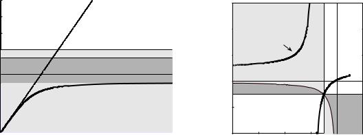
Case (a) ω0/ωp = 0.4. The variations of ε(ω) and μ(ω) as a function of frequency are shown in Fig. 3.30. The question we are asking now is what kind of surface modes may exist for this set of parameters. For simplicity we shall take εr1 = μr1 = 1, although the equations are valid for the case of a general lossless dielectric. It can be shown from eqns (3.76)–(3.79) that there are three SPP modes, as may be seen in Fig. 3.31(a). The first one is a TM mode that exists in the range 0 < ω < ω0. Thus, the presence of the magnetic resonance limits the range of the TM mode. Instead of moving up to ωs it stops now at ω0. In other words, the upper frequency limit occurs where μr2 turns negative instead of εr2 = −1. The second mode is a TE one that starts at the light line at a value of ω where εr2μr2 = 1 and tends asymptotically to the value of ω where μr2 = −1. It is a backward wave. The third mode is again a TM one. It starts at the same point as the TE mode but it moves upwards to tend asymptotically to the εr2 = −1 line. Not shown in the figure is the bulk mode that propagates for the range of frequencies for which both εr2 and μr2 are negative.
Let us now return to our diagram of Fig. 3.29 showing the areas in the εμ plane in which surface modes are possible. Each of our three modes may be represented by a curve in this plane replotted in Fig. 3.31(b). For the lower TM mode μ is positive and ε is negative. As ω varies from 0 to ω0 the curve denoted by (i) is described. As ω tends to ω0 we know that the permeability tends to infinity and then suddenly changes to minus infinity. Up to μ = ∞ there is a TM mode, but when the permeability switches to −∞ the surface mode is no longer there. As the frequency increases further the permeability now increases from minus infinity. At a certain value of the frequency it reaches the point P and then traverses a number of regions between P and Q. In the PA region, as may be seen from the shading, there cannot be surface modes.
114 Plasmon–polaritons
Z/Z p
1.6
1.4
1.2
1
0.8
0.6
0.4
0.2
0
0
|
|
|
line |
|
|
|
|
6 |
|
|
|
|
|
|
|
light |
|
|
|
|
|
|
|
|
|
|
|
|
|
|
|
|
P=0 |
|
4 |
|
|
|
|
|
|
|
|
|
|
|
|
|
|
|
|
|
|
|
|
|
|
|
|
|
|
H=0 |
|
|
|
(i) TM |
|
|
|
|
|
|
|
|
|
|
2 |
|
|
|
|
|
|
HP=1 |
|
|
|
(iii) TE |
|
P=−1 |
1 |
|
|
|
|
|
|
|
|
|
|
|
/P |
|
|
|
|
|
|
||
|
|
|
|
|
|
|
|
|
|
|
|
||
|
|
|
|
(ii) TM |
|
Z |
2 |
|
|
|
|
|
|
|
|
|
|
|
0 |
|
|
|
|
|
Q |
||
|
|
|
|
|
=PP |
|
|
|
|
|
|||
|
|
|
|
|
|
H=−1 |
|
|
|
|
|
||
|
|
|
|
|
|
|
|
|
|
|
|
||
|
|
|
|
|
|
|
0 |
|
|
|
|
|
|
|
|
(i) TM |
|
|
|
|
|
|
|
|
|
||
|
|
|
|
|
|
|
|
|
|
B |
|
||
|
|
|
|
|
|
|
|
|
|
|
|
|
|
|
|
|
|
|
|
|
|
−2 |
|
|
|
|
|
|
|
|
|
|
|
|
|
|
|
|
(ii) TM |
A |
(iii) TE |
|
|
|
|
|
|
|
|
−4 |
|
|
|
P |
|
0.5 |
1 |
|
1.5 |
2 |
2.5 |
3 |
|
−6 |
−4 |
−2 |
0 |
2 |
|
|
|
−8 |
|||||||||||
|
|
|
kx/kp |
|
|
|
|
|
|
H=H2/H1 |
|
|
|
(a ) |
(b ) |
Fig. 3.33 SPP dispersion for single interface. F = 0.56, ω0 = 0.8 ωp. (a) ω–kx diagram. (b) μ − ε diagram
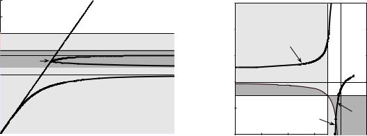
The TE region is entered at A and this mode exists until the frequency is high enough to reach B. This is the mode we have denoted by (ii). Increase ω again and we move from B to C, which is in the TM mode region corresponding to mode (iii). The curve continues beyond C as ω increases but no further surface modes are possible. It is interesting to note that this novel presentation in terms of geometrical loci in the ε,μ plane is not only capable of accounting for all the modes but also makes it clear how the various surface modes arise.
Next, let us consider what happens when ω0 increases, i.e. the magnetic resonance moves up in frequency. It may be shown that both the TE mode and the upper TM mode we have seen in Fig. 3.31(b) become flatter and then disappear altogether. For case (b), when ω0/ωp = 0.6 is taken, only the lower TM mode survives, as shown in the dispersion curve of Fig. 3.32(a). The geometrical locus of this TM mode in the εμ plane resembles the one in Fig. 3.31(b), but has shifted to the right, as illustrated in Fig. 3.32(b). What happened to the other two modes? Could we get our answer from the geometrical loci? What happened is that the PQ curve also moved to the right. At this particular value of ω0/ωp = 0.6 it crosses the ε = −1, μ = −1 point at A without ever crossing the area in which either surface mode exists.
When ω0 increases further there is an inversion of the upper TE and TM modes. First comes a backward TM mode and further up (although starting again at the same point) a forward TE mode. These changes are indicated by the next set of curves taken for ω0/ωp = 0.8 (Fig. 3.33). Note that ω0 > ωs, hence the magnetic resonance does not a ect the lower TM mode. Its range is, as in the case when μ is frequencyindependent, between ω = 0 and ω = ωs. The dispersion curves of the three modes are plotted in Fig. 3.33(a) and the corresponding curves in the ε,μ plane in Fig. 3.33(b). It may be clearly seen that in the interval