

Waves_in_Metamaterials
.pdf3.4 Surface plasmon–polaritons on a slab: TM polarization 95
|
0.5 |
|
|
|
|
|
|
|
Z(−) |
|
|
|
|
light |
|
|
|
|
|
|
|
|
|
|
|
|
(electrostatic) |
|
|
|
|
|
|
||
|
0.4 |
light |
|
|
|
|
light |
|
|
|
|
|
|
line |
|
|
|
|
|
Z(−) |
(electrostatic) |
|
|
|
|
|
|
|
|
|
|
||||
|
|
line |
|
line |
|
|
|
|
|
|
|
|
|
|
|||
|
|
|
|
|
|
|
|
|
|
|
|
|
|
|
|
|
|
p |
0.3 |
|
|
|
|
|
|
|
|
|
|
|
|
|
(−) |
(electrostatic) |
|
Z/Z |
|
|
|
|
|
|
|
|
|
|
|
|
|
|
Z |
|
|
0.2 |
|
|
|
|
|
|
|
|
Z(−) |
|
|
|
|
|
|
|
|
|
|
|
|
Z(−) |
|
|
|
|
|
|
|
|
|
Z(−) |
|
|
|
|
|
|
|
|
|
|
|
|
|
|
|
|
|
|
|
|
|
|
0.1 |
|
|
|
|
|
|
|
|
|
|
|
|
|
|
|
|
|
0 |
|
|
|
|
|
|
|
|
|
|
|
|
|
|
|
|
|
0 |
0.2 |
0.4 |
0.6 |
0.8 |
1 0 |
0.2 |
0.4 |
0.6 |
0.8 |
1 |
0 |
0 2 |
0.4 |
0.6 |
0.8 |
1 |
|
|
|
|
kx/kp |
|
|
|
|
kx/kp |
|
|
|
|
|
kx/kp |
|
|
|
|
|
|
(a) |
|
|
|
|
(b) |
|
|
|
|
|
(c) |
|
|
|
|
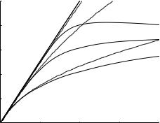
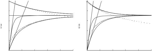
Fig. 3.19 (a) Electrostatic approximation and full solution for a slab. kpd = 0.25, 0.5, 1 (a)–(c) |
|
||||||||||||||
Two other approximations for small kx were first given by Economou (1969). The derivation is given below. For small enough kx we may expect the solution to be close to the light line, i.e. we may assume
k2 |
= k2 |
(1 + δ2) , |
(3.38) |
x |
0 |
|
|
where δ2 1. It follows then that
κ2 = kp |
and |
κ1 = δk0 . |
(3.39) |
We may then determine δ by substituting eqn (3.39) into eqn (3.35) yielding
δ = |
ω |
coth |
kpd |
, |
(3.40) |
|
|
||||
|
ωp |
2 |
|
|
|
which leads to the approximate dispersion equation
|
|
ωp |
|
2 |
|
|
|
|
2 |
|
|
kpd |
|
|
|
kx2 = k02 |
1 + |
ω |
coth2 |
|
. |
(3.41) |
|
2 |
|
|
|||||
If δ → ∞, i.e. we are back to the single interface, then the approximate curve is
k2 |
= |
ω2 |
+ |
ω4 |
. |
(3.42) |
||
c2 |
c2 |
ω2 |
||||||
x |
|
|
|
|
||||
|
|
|
|
|
p |
|
|
|
Note that eqn (3.41) would further simplify when kpd/2 1 to
k2 |
= |
ω2 |
+ |
4 |
|
ω4 |
. |
(3.43) |
|
|
2 |
2 |
4 |
||||||
x |
|
c |
|
|
|
||||
|
|
|
|
d |
|
ωp |
|
|
|
It can be immediately seen that the smaller d is the farther is the dispersion equation from the light line for a given ω. Next, we shall look for an approximation for the upper branch. We shall assume again that
96 Plasmon–polaritons
Fig. 3.20 Full solution and various approximations for a slab. kpd = 0.5
|
|
|
|
|
|
|
|
Z |
) |
|
) |
|
|
|
|
|
|
|
|
|
|
|
|
||
|
|
|
|
|
|
|
(low |
|
|
Z |
|
|
|
|
|
|
|
|
|
|
|
|
|
||
|
1 |
|
|
|
|
(+) |
|
|
|
(low |
|
|
|
|
|
|
|
|
|
|
|
|
|
||
|
|
|
|
|
Z |
|
|
|
|
|||
|
|
|
|
|
|
|
|d |
|
|
|||
|
|
|
line |
|
|
Z |
|
|
Z(+) |
|||
|
0.8 |
|
|
|
|
|
|
|
||||
|
light |
|
|
|
|
|
|
|
|
|
||
|
|
|
|
|
Z|d |
|
|
|
||||
|
|
|
|
|
|
|
|
|
||||
p |
0.6 |
|
|
|
|
|
|
) |
|
|
||
|
|
|
|
|
|
|
|
|
||||
Z |
|
|
|
|
) |
|
Z |
|
|
|
||
|
|
|
|
(low |
|
|
|
|
|
|||
/ |
|
|
|
|
|
|
|
|
|
|||
|
|
|
( |
|
|
|
|
|
|
|
Z( ) |
|
Z |
|
|
|
Z |
|
|
|
|
|
|
|
|
0.4 |
|
|
|
|
|
|
|
|
|
|
|
|
|
|
|
|
|
|
|
|
|
|
|
|
|
|
0.2 |
|
|
|
|
|
|
|
|
|
|
|
|
00 |
0.5 |
|
|
1 |
|
|
|
|
1.5 |
2 |
|
|
|
|
|
kx/kp |
|
|
|
|
|
|||
15We used an iterative technique first assuming the value of kx from the lossless solution and finding kx , and then for this value of kx finding the corresponding value of kx , etc.
kx is small and close to the light line so that we can start again with eqn (3.38). Then, using the same technique we find
δ = ωp tanh |
2 |
, |
|
(3.44) |
||||||||
|
ω |
|
|
kpd |
|
|
|
|
||||
leading to |
|
|
|
|
|
|
|
|
|
|
|
|
|
|
|
|
ωp |
|
|
|
2 |
|
|||
|
2 |
|
|
|
kpd |
|
|
|||||
kx2 = k02 1 + |
ω |
tanh2 |
|
, |
(3.45) |
|||||||
2 |
|
|
||||||||||
or after expanding the tanh function to |
|
|
|
|
|
|||||||
k2 |
= |
ω2 |
|
+ |
ω4d2 |
. |
|
(3.46) |
||||
c2 |
|
|
||||||||||
x |
|
|
|
4c4 |
|
|
|
|
||||
It may now be seen that the smaller d is the nearer is this branch of the dispersion equation to the light line.
Using the above-derived approximations for ω(−) and ω(+) we plot in Fig. 3.20 the approximate and exact curves for kpd = 0.5. The approximation is very good for small kx up to about ω/ωp = 0.35 and deteriorates afterwards.
So far we have looked at the lossless case but of course attenuation is equally important if we have practical applications in mind. We need to find not only the ω versus kx curve but also ω versus kx. How will kx enter our equations? It will be through κ2, which in the presence of losses will take the form
κ22 = (kx − j kx)2 + k02(ε − j ε ) . |
(3.47) |
We need to substitute κ2 from above into eqns (3.33) and (3.34) taking good care that ζe depends both on κ2 and on εr2. We are not aware of any analytical approximations for this case. We need to resort to numerical solutions.15
3.4 Surface plasmon–polaritons on a slab: TM polarization 97
|
|
Z(+) |
|
|
|
Z(−) |
|
|
0.6 |
|
|
|
|
|
|
|
kpd=0.25 |
|
|
|
|
|
|
|
|
|
|
|
|
|
|
p |
0.4 |
kpd=0.5 |
|
|
|
|
|
Z/Z |
|
|
k |
|
d |
kpd |
|
|
|
kpd=1 |
p |
kpd=1 |
|||
|
|
|
|
|
|||
|
|
|
|
|
|
||
|
0.2 |
|
|
|
|
|
kpd=0.5 |
|
|
|
|
|
|
|
|
|
|
|
|
|
|
|
kpd=0.25 |
|
|
|
10−5 |
|
100 |
10−5 |
100 |
|
|
|
kx"/kp |
|
|
kx"/kp |
|
|
|
|
(a) |
|
|
(b) |
|
|
|
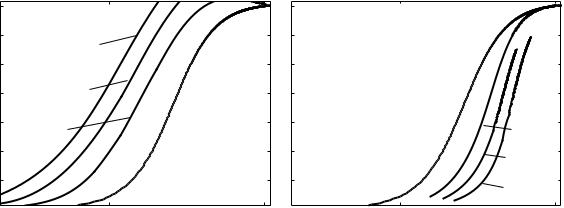
Fig. 3.21 Attenuation coe cient versus frequency for ω(+)-branch (a) and ω(−)-branch (b) |
|
||||
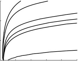
We shall not replot the frequency against normalized propagation constant curve—which remains practically the same. The frequency against normalized attenuation coe cient is plotted in Figs. 3.21(a) and (b) for the ω(+) and the ω(−) branches, respectively, for a range of normalized slab thicknesses. It may be seen that the waves in the upper branch are much less attenuated than the waves in the lower branch. In Fig. 3.22 we shall return to the concept of propagation length. It is plotted against the free-space wavelength for the ω(+) branch. It may be clearly seen that as the thickness declines, the propagation length increases. The reason why attenuation is lower for the upper branch is far from being obvious. We shall show first the field distributions and then discuss in quite some detail the physical reasons why the upper branch deserves the epithet of ‘long range’.
3.4.2Field distributions
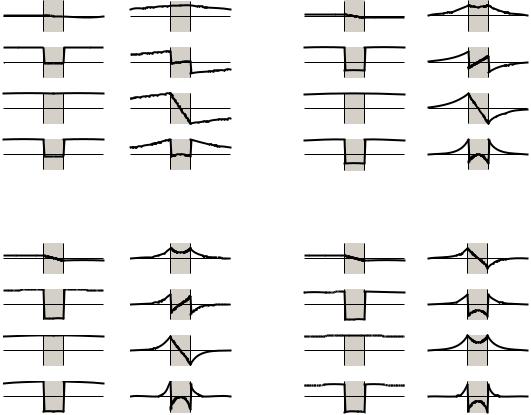
Let us now see the field distributions at one of these thicknesses (kpd = 0.25) for ω/ωp = 0.3, 0.5 and 0.7. They are plotted in Figs. 3.23(a)–
(c). Let us first look at the symmetry. For the upper mode Ez and Hy (and, consequently, Sx) are symmetric as a function of z, whereas Ex is antisymmetric. For the lower mode Ez and Hy are antisymmetric (consequently, Sx is symmetric) and Ex is symmetric. It is also true, as we have already known for the single interface, that the decay away from the interfaces becomes stronger as ω/ωp increases. It also follows from the figures that Sx is positive in the dielectric and flows in the opposite direction in the metal. As ω increases towards ωs the net power flow tends to zero. We need to emphasize that for a given ω up to ωs we had two di erent values of kx belonging to two di erent branches of
98 Plasmon–polaritons
Fig. 3.22 Propagation length versus free-space wavelength
|
100 |
d=10nm |
20nm |
|
|
|
[m] |
|
|
|
|
60nm |
|
10−2 |
|
|
|
100nm |
|
|
length |
|
|
|
|
|
|
|
|
|
|
d |
|
|
propagation |
10−4 |
|
|
|
|
|
|
|
|
|
free-space Of |
|
|
|
|
|
|
|
|
|
|
10−6 |
2 |
4 |
6 |
8 |
10 |
|
0 |
|||||
|
|
|
|
Of [Pm] |
|
|
the dispersion curve. Above ωs the situation is di erent. Although for a given value of ω there are still two values of kx, they happen to belong to the same branch, to the upper branch. The field distribution corresponding to ω/ωp = 0.735 is shown in Fig. 3.23(d). The symmetries are now the same at both values of kx: the fields Ez, Hy and the Poynting vector Sx are symmetric and Ex is antisymmetric. As we may also expect, the decay of the fields away from the metal is steeper for the higher kx. A good look at Sx will show (and numerical integration will prove it) that the total power carried is now in the opposite direction. The wave is a backward wave.
As we have seen, a field distribution is either symmetric or antisymmetric. So terminology should be easy: those that have symmetric distribution should be called symmetric modes and denoted by s, and those with antisymmetric distribution could be called antisymmetric (or asymmetric) modes and denoted by a. The problem is which field component should we refer to? Is it Ez, the field component normal to the direction of propagation, or Ex the field component in the direction of propagation? Opinions have been divided. Economou (1969) refers to the lower branch, ω(−), as that with symmetric oscillation and to the upper branch as that with antisymmetric oscillation. For him it is the charge distribution, and the e ect of the tangential component of the electric field on it, that is of primary importance. Burke et al. (1986) call the upper branch symmetric and the lower branch antisymmetric. According to Welford (1988), in the upper branch the two surface waves propagate π out of phase and hence should be referred to as the antisymmetric mode. In the branch with the lower ω the surface waves propagate in phase and should therefore be referred to as the symmetric mode. Burke et al. (1986) attributed the conflict in notations to the di erent background of the authors. The terminology in which the antisymmetric mode has a zero in its transverse electric field inside the film comes from integrated optics and is just opposite to the solid-state version, which
Z(+)
Ex
Ez
Hy
Sx
Z(+)
Ex
Ez
Hy
Sx
3.4 Surface plasmon–polaritons on a slab: TM polarization 99
Z(−)
Ex
Ez
Hy
Sx
(a)
Z(−)
Ex
Ez
Hy
Sx
Z(+) |
Z(−) |
E |
Ex |
x |
|
Ez |
Ez |
|
|
Hy |
Hy |
|
|
Sx |
Sx |
|
|
|
(b) |
Z(+) |
Z(+) |
Ex |
E |
|
x |
Ez
Ez
Hy
Hy
Sx
Sx
(c) |
(d) |
Fig. 3.23 Field distributions of ω(+) and ω(−)-branches for four typical frequencies (a)–(d) ω/ωp = 0.3, 0.5, 0.7, 0.735
deals with the symmetries of the charge distribution and therefore with the longitudinal components of the electric field. By now it has been largely accepted16 that the mode in which the normal component of the electric field is symmetric is denoted by s and that in which the normal component is antisymmetric is called a. In addition, when the waves are bound the modes are referred to as sb and ab and when they are leaky17 as sl and al.
If the metal is lossless the modes are lossless. If the metal is lossy the modes are lossy, so much is clear. But which one is lossier? The calculations show that the sb mode is less lossy, meriting the description of ‘long-range surface plasmon’. We shall show curves later but first let us try to give a physical explanation.
One explanation may be based on the fact that the ω(+)-mode is nearer to the light line. If it is nearer it resembles more an electromagnetic wave. Electromagnetic waves travel in vacuum with no attenuation, hence the upper branch will be the one that has the lower attenuation.
16Maier et al. (2005) use a notation somewhat at variance with the usual
notions of symmetry and antisymmetry. They refer to the ω(+)-mode
as ‘antisymmetric (sb) mode’ and to the ω(−)-mode as the ‘symmetric (ab ) mode’.
17Leaky waves, as the name implies, leak out power, which is good for antennas but not for guiding the wave. Here, we are concerned only with bound modes so, with regret, we shall not discuss the properties of leaky waves.

100 Plasmon–polaritons
Mansuripur et al. (2007) o ers a somewhat more complicated explanation for the loss mechanism. With the even mode, the field component Ez has the same sign on the boundaries of the slab; therefore at a given point along x, the electrical charges on the upper and lower surfaces have opposite signs. Inside the metallic slab, the field component Ez— reduced by a factor εr2/εr1 relative to the Ez immediately outside— helps move the charges back and forth between the two surfaces. The slab being thin, the transport distance is short; hence the corresponding electrical current is small. In contrast, the charges of the odd mode have the same sign on opposite sides of the slab. Consequently, positive and negative charges must move in the x direction during each period of oscillation. The travel distance is now of the order of the SPP wavelength, which is greater than the slab thickness. Therefore, the current densities of the odd mode are relatively large, leading to correspondingly large losses.
A fairly similar reasoning is due to Zayats et al. (2005) giving the Ex component as being responsible for loss. For the ω(+) mode Ex vanishes at the midplane of the slab, while it is a maximum at that plane for the ω(−) mode. The mode with the smaller fraction of the electric field inside the metal causes less dissipation.
Barnes (2006) explains the loss mechanism as follows. The ω(+) mode propagates in such a way that less of the power is carried in the metal than in the case of a single-interface mode. This reduces the e ect of loss. Propagation lengths of the order of centimeters may be achieved. There is though a price to pay for such long propagation: the mode is not localized at the surface, it extends further into the dielectric, resembling the transverse plane electromagnetic wave.
Maybe the best explanation is based on the penetration depth in the metal. It may be seen in Figs. 3.23(a)–(c) that for a given frequency the antisymmetric mode at the higher kx has a fast decay away from the metal surface. The symmetric mode has a slower decay, hence more field is in the dielectric, consequently, it is less lossy.
Another consideration is confinement of the fields. The more they are confined, the larger they are and that’s a good thing for applications in which high fields are required. On the other hand, as the arguments above have shown, confinement leads to higher losses. Hence, some compromise between the two must always be made. For a discussion of the trade-o see Berini (2006).
H3 |
Dielectric |
|
|
H2 |
Metal |
|
d |
|
|||
|
|
|
|
H1 |
Dielectric |
|
|
|
|
|
|
Fig. 3.24 Metallic slab surrounded by di erent dielectric media
3.4.3Asymmetric structures
We use here the terms symmetric and asymmetric in yet another sense, referring this time to structures. A symmetric structure is when the dielectrics on the two sides of the metal slab are identical and it is asymmetric when the dielectrics are di erent (see Fig. 3.24).
The asymmetric structure was investigated in some of the early papers (Sarid, 1981; Wendler and Haupt, 1986; Burke et al., 1986; Yang et al., 1991) but received much less attention than the symmetric case. If there

3.4Surface plasmon–polaritons on a slab: TM polarization 101
|
|
|
|
|
|
|
|
|
|
|
|
|
|
|
|
|
|
|
|
|
|
|
|
103 |
|
|
|
Ag |
|
|
|
|
|
a=10 nm |
|
|
|
|
|
|
|
||||
|
|
|
|
|
|
|
|
|
|
|
|
|
|
|||||||||
|
|
|
|
O=632.8 nm |
|
|
|
|
|
|
|
|
|
|
|
|||||||
|
|
|
|
|
|
|
|
|
|
|
|
|
|
|
17 nm |
|
|
|
|
|
|
|
|
102 |
|
|
|
|
|
|
|
|
|
|
|
|
|
30 nm |
|
|
|
|
|
|
|
L (cm) |
|
|
|
|
|
|
|
|
|
|
|
|
|
50 nm |
|
|
|
|
|
|
|
|
|
|
|
|
|
|
|
|
|
|
|
|
|
|
|
|
|
||||||
|
|
|
|
|
|
|
|
|
|
|
|
|
|
|
|
|
|
|
|
|||
101 |
|
|
|
|
|
|
|
|
|
|
|
|
|
|
|
|
|
|
|
|
|
|
length |
|
|
|
|
|
|
|
|
|
|
|
|
|
|
|
|
|
|
|
|
|
|
|
|
|
|
|
|
|
|
|
|
|
|
|
|
|
|
|
|
|
|
|
||
|
|
|
|
|
|
|
|
|
|
|
|
|
|
|
|
|
|
|
|
|
|
|
Propagation |
100 |
|
|
|
|
|
|
|
|
|
|
|
|
|
|
|
|
|
|
|
|
|
|
|
|
|
|
|
|
|
|
|
|
|
|
|
|
|
|
|
|
|
|
|
|
|
10–1 |
|
|
|
|
|
|
|
|
|
|
|
|
|
|
|
|
|
|
|
|
|
|
|
|
|
|
|
|
|
|
|
|
|
|
|
|
|
|
|
|
|
|
|
|
|
10–2 |
|
|
|
|
|
|
|
|
|
|
|
|
|
|
|
|
|
|
|
|
Fig. 3.25 Propagation length of the |
|
|
|
|
|
|
|
|
|
|
|
|
|
|
|
|
|
|
|
|
|
||
|
|
|
|
|
|
|
|
|
|
|
|
|
|
|
|
|
|
|
|
|
|
|
|
|
|
|
|
|
|
|
|
|
|
|
|
|
|
|
|
|
|
|
|
|
long-range SPP vs. dielectric constants |
|
|
|
|
|
|
|
|
|
|
|
|
|
|
|
|
|
|
|
|
|
|
εr1 of the superstrate and εr3 of the |
|
1.9 |
2.0 |
2.1 |
|
2.2 |
2.3 |
2.4 |
|||||||||||||||
|
|
substrate for di erent thicknesses a of |
||||||||||||||||||||
|
|
|
|
|
|
|
|
|
|
|
|
|
|
|
|
|
|
|
|
|
|
|
|
Hr1 Hr3 = 2.1211) |
Hr1 |
|
Hr3 Hr3 Hr1 |
= 2.1211) |
|
the Ag layer. From Wendler and Haupt |
|||||||||||||||
|
|
|
||||||||||||||||||||
|
|
|
(1986). Copyright c 1986 American |
|||||||||||||||||||
|
|
|
|
|
|
|
|
Dielectric constants |
|
|
|
|
|
|
||||||||
|
|
|
|
|
|
|
|
|
|
|
|
|
|
Institute of Physics |
||||||||
is only a small di erence in the dielectric constant then we can still talk about quasi-symmetric and quasi-antisymmetric modes but we find that the field confinement is very asymmetric. The quasi-symmetric mode is localized at the boundary between the metal and the dielectric with the lower dielectric constant, whereas the quasi-antisymmetric mode is localized at the higher dielectric constant boundary. The quasi-symmetric mode inherits the mantle of the sb mode: it is still the long-range mode, it still has a lower attenuation and, as may be expected, the attenuation decreases as the slab thickness decreases. The new phenomenon is that the quasi-symmetric mode has a cuto thickness below which no propagation is possible. This is bound to occur (Berini, 2001) because the sb mode no longer has the chance quietly to convert into the TEM electromagnetic wave as d → 0 because the di erent dielectrics on the two sides do not permit it. The quasi-antisymmetric mode remains the short-range mode, its attenuation increases with decreasing slab thickness, it has not got a cuto thickness.
For detailed calculations of the propagation length in asymmetric structures see Wendler and Haupt (1986). They investigate theoretically thin silver slabs at the He-Ne wavelength of 632.8 nm with a dielectric constant of εr2 = −18−j 0.47 obtained from Johnson and Christy (1972). They first assume that both dielectrics have identical dielectric constants of εr1 = εr3 = 2.1211, then change the dielectric constant of one of them within a range of about 20%. They find that the propagation length first remains unchanged and then suddenly increases. Their
102 Plasmon–polaritons
results, quite spectacular, are shown in Fig. 3.25.
In a further study Zervas (1991) showed that long-range SPPs are supported even by highly asymmetric configurations.
3.5Metal–dielectric–metal and periodic structures
It is now an easy exercise to derive dispersion for the surface modes for a thin dielectric layer with two semi-infinite metallic media adjacent to it. The dispersion equations are very similar to those of eqns (3.35) and (3.36) and can be derived in an analogous manner. In the final result the only di erence is that κ2 is being replaced by κ1 in the arguments of the tanh and coth functions, i.e. the equations are given as
ζe = −tanh |
κ1d |
, |
(3.48) |
|
2 |
|
|||
and |
|
|
|
|
ζe = −coth |
κ1d |
|
|
|
|
. |
(3.49) |
||
2 |
||||
As before, we shall try to find some approximations. For the upper branch ω(+) we can take the argument of the coth function small and
then without further approximations we find |
− |
|
|
|
|
||||||||||
kx2 = |
d |
|
2 |
1 − ωp |
|
ω |
|
− ω |
2 |
. (3.50) |
|||||
|
2 |
|
|
|
ω |
|
ωp |
4 |
|
ωp |
2 |
kpd |
|
|
|
The frequency at which kx = 0 may be obtained from the above equation as
ω |
= 1 − |
1 |
(kpd)2 , |
(3.51) |
|
|
|||
ωp |
8 |
i.e. the dispersion curve cuts the vertical axis just below the bulk plasma frequency.
We may again resort to the electrostatic approximation that turns out to be identical with that (eqn (3.36)) already derived for the dielectric– metal–dielectric structure.
The dispersion curves calculated from eqns (3.48) and (3.49) are plotted in Figs. 3.26(a) and (b) together with the electrostatic approximation and that given by eqn (3.50) for kpd = 0.25 and 0.5. The first thing to notice is that the ω(+) branch crosses the light line. The wave can propagate at phase velocities higher than the velocity of light. The ω(−) branch behaves as it did for the dielectric–metal–dielectric structure. It tends to ωs for kx → ∞ and to the light line as kx → 0. The electrostatic approximation is quite good for the ω(−) mode and even better for the ω(+) mode. The low kx approximation, not surprisingly, deteriorates as kx increases.
3.6 One-dimensional confinement: shells and stripes 103
|
|
|
|
|
|
|
|
|
|
|
|
|
|
|
|
|
|
|
|
|
) |
|
|
|
|
|
|
|
|
|
|
|
|
|
|
|
|
|
|
|
|
|
|
|
|
|
|
|
|
|
|
|
|
Z |
|
|
|
|
|
|
|
|
|
|
|
|
|
|
|
|
|
|
|
|
|
|
|
|
|
|
|
|
|
|
|
(low |
− |
|
|
|
|
|
|
|
|
|
|
|
1 |
|
|
|
|
|
|
|
|
|
|
|
|
|
|
|
|
1 |
|
) |
|
|
|
|
|
|
|
|
|
|
|
|
|
|
|
|
|
|
|
|
|
|
|
|
|
|
|
|
|
|
|
|
|
|
|
|
|
|
|
|
|
|
|
|
|
|
|
|
|
|
|
|
|
|
|
|
|
|
|
|
|
|
|
|
|
− |
|
|
|
|
|
|
|
|
|
|
|
|
|
|
|
|
|
|
|
|
(+) |
|
|
|
|
|
|
|
|
|
|
( |
|
|
|
|
|
|
|
|
|
|
|
|
|
|
|
|
|
|
|
|
Z |
(el.- |
|
|
|
|
|
|
|
Z |
|
|
|
(+) |
|
|
|
|
|
|
|
|
|||||
|
|
|
|
|
|
|
|
|
|
|
|
|
|
|
|
|
|
|
|
|
|
|
|
|
|
|
|
|
||||
|
line |
|
|
|
|
|
|
|
|
|
stat.) |
|
|
(+) |
|
|
|
|
|
|
Z |
|
(el.- |
|
|
|
|
|
|
|
||
0.8 |
|
|
|
|
|
|
(+) |
(low− |
|
|
|
|
0.8 |
line |
|
|
|
|
|
|
stat.) |
|
|
|
(+) |
|
|
|||||
|
|
|
|
Z |
Z) |
|
Z |
|
|
|
|
|
|
|
|
|
|
|
|
|
||||||||||||
|
light |
|
|
|
|
|
|
|
|
|
|
|
|
|
|
|
|
|
|
|
|
|
|
|
|
|
|
|
||||
|
|
|
|
|
|
|
|
|
|
|
|
|
|
light |
|
|
|
|
|
|
|
|
Z |
|
|
|
|
|||||
|
|
|
|
|
|
Z| |
|
|
|
|
|
|
|
|
|
|
|
|
|
|
|
|
|
|
|
|
|
|||||
|
|
|
|
|
|
|
|
|
|
|
|
|
|
|
|
|
|
|
|
.) |
|
|
|
|
|
|
|
|||||
|
|
|
|
) |
|
|
|
|
d |
|
|
|
|
|
|
|
|
|
|
|
|
stat |
|
|
(+) |
|
|
|
||||
|
|
|
|
Z |
|
|
|
|
|
|
|
|
|
(−) |
|
|
|
|
|
|
.- |
|
|
|
|
|
|
|||||
0.6 |
|
|
|
|
|
|
|
|
|
|
|
|
|
0.6 |
|
|
)(el |
|
|
|
|
Z |
|
|
(low− |
|
|
|||||
|
|
|
− |
|
|
|
) |
|
|
|
|
Z |
|
|
|
( |
|
|
|
|
|
|
|
|
|
|
|
) |
||||
p |
|
|
(low |
|
|
|
|
. |
|
|
|
|
|
|
|
|
p |
|
|
|
|
|
|
|
|
|
|
|
|
|
Z |
|
|
|
|
|
stat |
|
|
|
|
|
|
|
|
|
Z |
|
|
|
|
|
|
|
|
|
|
|
|
||||||
|
|
|
|
.- |
|
|
|
|
|
|
|
|
|
|
|
|
|
|
|
|
|
|
|
|
|
|
|
|
|
|
||
|
|
|
) |
|
|
|
|
|
|
|
|
|
|
|
|
|
|
|
|
|
|
|
|
|
|
|
|
|
|
|
||
/ |
|
) |
(− |
(el |
|
|
|
|
|
|
|
|
|
|
|
/ |
|
|
(−) |
|
|
|
|
|
|
|
|
|
|
|
||
|
|
|
|
|
|
|
|
|
|
|
|
|
|
|
|
|
|
|
|
|
|
|
|
|
|
|||||||
|
Z |
|
|
|
|
|
|
|
|
|
|
|
|
|
|
|
|
|
|
|
|
|
|
|
|
|
||||||
|
|
− |
|
|
|
|
|
|
|
|
|
|
|
|
|
|
|
|
Z |
|
|
|
|
|
|
|
|
|
|
|
|
|
0.4 |
|
( |
|
|
|
|
|
|
|
|
|
|
|
|
|
|
0.4 |
|
|
|
|
|
|
|
|
|
|
|
|
|
|
|
|
Z |
|
|
|
|
|
|
|
|
|
|
|
|
|
|
|
|
|
|
|
|
|
|
|
|
|
|
|
|
|
||
0.2 |
|
|
|
|
|
|
|
|
|
|
|
|
|
|
|
|
0 2 |
|
|
|
|
|
|
|
|
|
|
|
|
|
|
|
0 |
|
|
|
2 |
|
|
|
|
4 |
|
6 |
8 |
|
10 |
0 |
|
|
2 |
|
|
|
4 |
6 |
|
8 |
|
|
10 |
||||
|
|
|
|
|
|
|
|
|
0 |
|
|
|
|
|
|
|
|
|||||||||||||||
|
|
|
|
|
|
|
|
|
|
|
kx/kp |
|
|
|
|
|
|
|
|
|
|
|
|
kx/kp |
|
|
|
|
|
|
|
|
|
|
|
|
|
|
|
|
|
|
|
(a) |
|
|
|
|
|
|
|
|
|
|
|
|
(b) |
|
|
|
|
|
|
|
|
Fig. 3.26 Dispersion curves for a metal–dielectric–metal structure. Full solutions and approximation for (a) kpd = 0.25 and |
||||||||||||||||||||||||||||||||
(b) kpd = 0.5 |
|
|
|
|
|
|
|
|
|
|
|
|
|
|
|
|
|
|
|
|
|
|
|
|
|
|
|
|
|
|
||
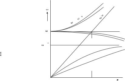
Economou (1969) goes on investigating two and more metal slabs between dielectrics, including the generalization to a periodic structure (see Fig. 3.27(a)). More and more layers in the structure lead to multiple splitting, i.e. to the appearance of more and more dispersion curves with the final result that both the ω(+) and the ω(−) branches widen into bands, as shown schematically in Fig. 3.27(b).
3.6One-dimensional confinement: shells and stripes
All the problems we have investigated so far have been concerned with two-dimensional confinement of the surface waves, to a single surface or to multiple surfaces. Clearly, for any practical application we need a one-dimensional structure to take information from point A to point B. Such a structure was analyzed by Al-Bader and Imtar (1992). They considered a cylindrical metallic shell of inner radius a, and thickness t embedded in a dielectric or in two di erent dielectrics. They set up the di erential equations for the fields of a TM mode and solved them numerically for silver at the He-Ne wavelength of 633 nm. They presented their results in terms of a mode index ne = ne − j ne where the complex propagation coe cient is given as k = k0ne. Their results were similar to those found for planar structures to which they reduced in the limit of infinite radius. They were also interested in the evolution of the TM01 fibre mode into surface plasmons, the model they considered was a dielectric cylinder embedded in metal. They found that the surface
104 Plasmon–polaritons
2 
2 p
2 2k
C
II a
ck
Metal |
|
|
|
|
|
|
|
|
|
Dielectric |
p |
|
|
|
|
|
II b |
||
|
|
I |
|
|
|
|
|
||
|
|
|
|
|
|
|
|||
|
p/ 2 |
|
|
|
|
max |
|
|
|
|
|
|
|
|
|
|
|||
|
|
|
|
|
|
|
|||
|
|
|
|
|
|
|
|
|
|
|
|
|
|
|
|
|
|
|
|
|
|
|
C |
|
|
||||
|
|
|
|
|
|
|
|
|
|
|
|
IV |
|
|
|
|
|
|
|
|
|
|
|
|
min |
|
|
||
|
|
|
|
|
|
|
|
||
|
III |
C |
|
|
|||||
|
|
|
|
|
|||||
|
|
|
|
|
|
|
|
||
|
O |
|
|
|
|
kp |
|
k |
|
|
|
||||||||
(a) |
|
|
|
|
|
|
(b) |
|
|
Fig. 3.27 Multilayer metal–dielectric structure. (a) Sketch of the configuration. (b) Dispersion relations. From Economou (1969). Copyright c 1969 by the American Physical Society
mode appeared for su ciently large radius.
The physics for cylindrical structures is quite similar to that of planar structures. However, a host of new phenomena appear when the infinite slab is turned into the one-dimensional metal stripe of width w and thickness t, as shown in Fig. 3.28(a). They have received considerable attention lately (Berini, 1999; Berini, 2000a; Berini, 2000b; Berini, 2001; Berini, 2006; Al-Bader, 2004) due to their promise of signal processing in the visible and infra-red region. They solved the relevant partial di erential equations subject to the boundary conditions by the method of lines. The main di erence they found relative to the 2D case was the variety of field distributions that could occur. Simple TM modes no longer exist. All six field components must be present in all modes. The question then arises as to what nomenclature to use to identify the modes. The obvious start (Berini, 1999; Berini, 2000a) is with the sb and ab modes of 2D structures because the symmetry of the 1D structure will again permit symmetric and antisymmetric modes, in fact there are two symmetry axes in the x and y directions of Fig. 3.28(a). When w/t 1 then the main transverse electric field is Ez whose symmetry with respect to the y and z axes is reflected in the use of the subscripts ss, sa, as, aa. A further superscript is then used to track the number of extrema observed in the spatial distribution of Ez along the y axis, and a second superscript would describe the extrema in the z direction (likely to exist but they have not been found so far). They are all bound modes, hence the subscript b is also added as for the 2D case. The new feature is that the higher-order modes have a cuto width below