

Waves_in_Metamaterials
.pdf3.7 SPP for arbitrary ε and μ 115
Z/Z p
1.6 |
|
|
|
|
|
P=0 |
6 |
|
|
|
|
|
|
|
|
|
line |
|
|
|
|
|
|
|
|||
|
|
|
|
|
|
|
|
|
|
|
|||
1.4 |
|
light |
|
|
|
|
|
|
|
|
|
||
1.2 |
|
|
|
(iii) TE |
P=−1 |
4 |
|
|
|
|
|
||
|
|
|
|
|
|
|
|
|
|
|
|||
1 |
H=0 |
|
|
|
|
|
|
|
(i) TM |
|
|
|
|
|
|
|
|
Z |
|
|
|
|
|
|
|||
|
|
|
|
|
0 |
2 |
|
|
|
|
|
||
|
|
|
|
|
|
1 |
|
|
|
|
|
||
0.8 |
|
|
|
|
|
/P |
|
|
|
|
|
|
|
|
|
|
|
|
2 |
|
|
|
|
|
Q |
||
|
|
|
|
|
|
=PP |
|
|
|
|
|
||
|
|
|
|
|
(i) TM |
H=−1 |
0 |
|
|
|
|
|
|
0.6 |
|
|
|
|
|
|
|
|
|
|
|||
|
|
|
|
|
|
|
|
|
|
A |
|||
|
|
|
|
|
|
|
|
|
|
|
|
||
0.4 |
|
|
|
|
|
|
−2 |
|
|
|
|
|
|
0.2 |
|
|
|
|
|
|
|
|
|
|
(iii) TE |
||
|
|
|
|
|
|
|
|
|
|
|
|||
0 |
|
|
|
|
|
|
−4 |
|
|
|
|
P |
|
0.5 |
1 |
1.5 |
2 |
2.5 |
3 |
−6 |
−4 |
−2 |
0 |
2 |
|||
0 |
−8 |
||||||||||||
|
|
|
kx/kp |
|
|
|
|
|
H=H2/H1 |
|
|
||
(a ) |
(b ) |
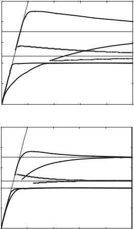
Fig. 3.34 SPP dispersion for single interface. F = 0.56, ω0 = ωp. (a) ω–kx diagram. (b) μ–ε diagram
PA we have a TM mode, between A and B a TE mode, and no surface mode beyond B.
In case (d) we have chosen ω0/ωp = 1. There is now no region for which μ and ε are simultaneously negative. The lower TM mode, as may be expected, remains unchanged. The upper TM mode has disappeared and only one TE mode remains in the frequency region where the permeability is negative. The dispersion curve is shown in Fig. 3.34(a) and the geometrical locus of the modes in Fig. 3.34(b). The region PA is now responsible for the upper TE mode and no surface mode exists beyond A.
We may summarize at this point the rules governing the appearance of the upper TM and TE modes. The upper TM mode exists in the frequency range between the values that give εμ = 1 and that giving ε = −1. Depending on which one is higher for the particular value of ω0/ωp it is a forward wave or a backward wave. When those two limits take identical values the upper TM mode disappears. The upper TE mode originates at the same point as the upper TM mode and tends asymptotically to the line μ = −1. Depending again on the relative positions of these two points the TE wave is a backward wave or a forward wave or it just vanishes when it changes from one into the other one.
Concerning the number of modes for a given value of ω0/ωp they vary between one and three. Specifically, there is only one mode for case (b), two modes for case (d), and three modes for cases (a) and (d). Case (a) has been considered by Ruppin (2001). Case (b) includes the perfect lens condition ε = μ = −1 at ω = ωs.
Note that the total number of modes is dictated by the chosen form for the frequency dependence of ε and μ that result in various ways of crossing the regions in which surface modes are allowed. A di erent
116 Plasmon–polaritons
Fig. 3.35 SPP dispersion for a slab. F = 0.56, ω0 = 0.4 ωp. kpd = 0.25 (a) and 1 (b)
1 |
|
line |
|
|
|
|
|
H |
|
|
|
|
|
|
(iii) TM |
Z(+) |
|
|
|
0.8 |
|
light |
|
|
|
|
|
|
|
|
|
|
|
|
|
|
|
H |
|
0.6 |
|
(ii) TE |
Z(+) |
|
|
Z(−) |
|
|
|
|
|
|
|
|
|
||||
p |
|
|
|
|
|
|
|
|
(a) |
ZZ |
|
|
|
|
Z(−) |
|
|
|
|
|
|
|
|
|
|
P |
|
||
0.4 |
|
Z(+) |
|
|
|
|
|
Z |
0 |
|
|
|
|
|
|
|
|||
|
|
|
|
|
|
|
|
||
0 2 |
|
(i) TM |
Z(−) |
|
|
|
|
|
|
|
|
|
|
|
|
|
|
|
|
0 |
|
|
1 |
2 |
3 |
4 |
|
5 |
|
0 |
|
|
|
||||||
|
|
|
|
kx/kp |
|
|
|
|
|
1 |
|
line |
|
|
|
|
|
H |
|
|
|
|
|
|
|
|
|
||
|
|
|
|
|
|
|
|
|
|
0.8 |
|
light |
|
|
|
(iii) TM |
Z(+) |
|
|
|
|
|
|
|
|
|
|
|
|
|
|
|
|
|
|
|
(−) |
H |
|
|
|
|
|
|
|
|
Z |
|
|
0.6 |
|
|
|
|
|
|
|
|
|
p |
|
|
|
(ii) TE |
Z(+) |
|
|
|
(b) |
ZZ |
|
|
|
|
|
|
|||
|
|
|
|
|
Z(−) |
|
P |
|
|
|
|
|
|
|
|
|
|
||
0.4 |
Z(+) |
(i) TM |
|
(−) |
|
|
|
Z0 |
|
|
|
Z |
|
|
|
|
|
|
|
0.2 |
|
|
|
|
|
|
|
|
|
0 |
|
|
1 |
2 |
3 |
4 |
|
5 |
|
0 |
|
|
|
||||||
|
|
|
|
kx/kp |
|
|
|
|
|
frequency dependence for ε and μ (e.g. with multiple resonances) can result in a smaller or larger number of modes. The results of Section 3.7.2 summarized in Fig. 3.29 would still apply.
A number of authors looked at di erent possibilities for the dependence of ε and μ on frequency. The results reported by Ruppin 2000; Darmanyan et al. 2003 can be reproduced with our model.
3.7.4SPP modes for a slab of a metamaterial
The story is the same again as for the epsilon-negative-only medium. If the slab is su ciently thin the modes on each side are coupled to each other. As a consequence, the number of branches in the dispersion equation of a slab will double in comparison to the single interface. Each mode splits into a symmetric and an antisymmetric branch. We take here only two examples, case (a) and case (b) of the previous section, i.e. for ω0 = 0.4ωp and ω0 = 0.6ωp. The resulting dispersion curves for
1 |
line |
|
|
|
|
|
|
|
H |
|
|
|
|
|
|
|
|
|
|
|
|
|
|
0.8 |
light |
(ii) TE |
Z(+) |
|
|
(iii) TM |
Z(+) |
|
|
|
|
|
|
|
|
|
|
|
|
|
|||
|
|
|
Z( |
) |
|
|
|
|
H P |
|
|
|
|
|
|
|
|
Z(−) |
|
|
|
||
0.6 |
|
|
|
|
|
|
|
Z0 |
|
|
|
p |
Z(+) |
|
|
|
|
|
|
|
|
(a) |
|
ZZ |
|
|
|
|
|
|
|
|
|||
|
|
|
|
|
|
|
|
|
|
|
|
0.4 |
|
(i) TM |
Z(−) |
|
|
|
|
|
|
|
|
|
|
|
|
|
|
|
|
|
|
||
0 2 |
|
|
|
|
|
|
|
|
|
|
|
0 |
|
2 |
|
4 |
6 |
8 |
10 |
|
|
||
0 |
|
|
|
|
|||||||
|
|
|
|
|
|
kx/kp |
|
|
|
|
|
1 |
line |
|
(ii) TE |
|
(iii) TM |
|
|
H |
|
|
|
|
|
|
|
|
|
|
|
||||
|
(+)} |
|
(+)} |
|
|
|
|
|
|||
|
light |
|
|
|
|
|
|
||||
0.8 |
Z |
Z(−) |
Z |
Z(−) |
|
|
|
|
|
||
|
|
|
|
|
|
|
|
|
|
|
|
|
|
|
|
|
|
|
|
|
H P |
|
|
0.6 |
|
|
|
|
|
|
|
|
Z |
|
|
|
|
|
|
|
|
|
|
0 |
|
||
p |
|
|
|
|
|
|
|
|
|
||
|
Z(+) |
|
|
|
|
|
|
|
|
|
|
ZZ |
|
|
|
|
|
|
|
|
|
(b) |
|
|
Z(−) }(i) TM |
|
|
|
|
|
|
|
|||
0.4 |
|
|
|
|
|
|
|
|
|||
|
|
|
|
|
|
|
|
|
|
|
|
0 2 |
|
|
|
|
|
|
|
|
|
|
|
0 |
|
|
|
|
|
|
|
|
|
|
|
0 |
|
2 |
|
|
4 |
6 |
8 |
10 |
|
|
|
|
|
|
|
|
|
kx/kp |
|
|
|
|
|
3.7SPP for arbitrary ε and μ 117
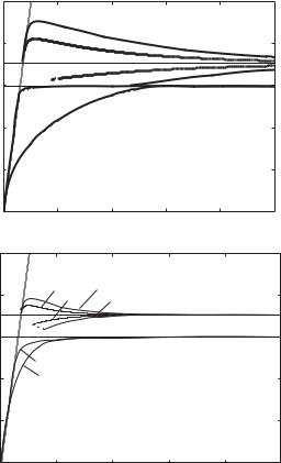
Fig. 3.36 SPP dispersion for a slab.
F = 0.56, ω0 = 0.6 ωp. kpd = 0.25 (a) and 1 (b)
kpd = 0.25 and 1.0 are shown in Figs. 3.35(a) and (b) and Figs. 3.36(a) and (b). Comparing them to the unperturbed solutions for the single interface shows some striking features in case (b). Apart from the low-ω TM, which splits into two, two further modes, a backward and a forward one, appear that asymptotically approach the miraculous frequency at which εr = μr = −1. The higher kx is, the closer are the two modes (one above and one below) to the single interface curve. Due to the di erent character of the frequency dependence of ε and μ, the split between the TE modes looks di erent from the split between the TM modes (it is actually larger for TM). We will return to this case later when discussing subwavelength imaging properties of the perfect lens.
The asymmetric structure when the two media surrounding the slab are di erent were first considered by Ruppin (2001) and later generalized by Tsakmakidis et al. (2006).
We finish this section by mentioning an idea due to Oulton et al. (2008). The authors note that, due to losses and stringent fabrication requirements, practical SPP waveguides have not succeeded in producing field confinement beyond that of dielectric waveguides. The new idea
118 Plasmon–polaritons
is to form a hybrid waveguide between a cylindrical dielectric nanowire and a metallic plate. In that case much of the power will propagate in the space between the nanowire and the plate, reducing thereby the losses, and confinement will be determined by the distance between them, which can be made very small by available semiconductor fabrication techniques. For further comments on this waveguide see Maier (2008).