

БЭМЗ полищук доки / 2020 / А2000 минск / Стандарт MIL-STD-202G
.pdfMIL-STD-202G
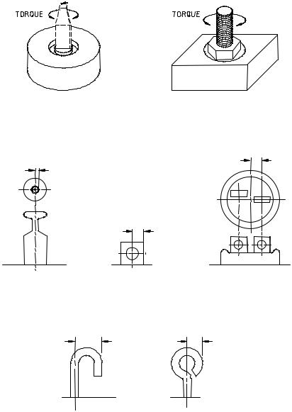
FIGURE 211-1. Test condition A.
FIGURE 211-2. Test condition B.
FIGURE 211-3. Test condition C.
METHOD 211A
14 April 1969
5

MIL-STD-202G
STEP 1. Bend lead with fingers, over rounded edge of metal plate as shown in (a). STEP 2. Center component part in chuck; secure lead in clamp as shown in (b).
STEP 3. Rotate chuck part through 360° at a rate of approximately 5 seconds per 360° rotation. Successive rotations shall be in alternate directions. A total of three such 360° rotations shall be performed. During this test, the chuck shall rotate around an axis which is fixed with respect to the padded clamp, or vice versa. The chuck shall have no appreciable end play during rotation.
NOTE: Metric equivalents are in parentheses.
FIGURE 211-4. Test condition D.
METHOD 211A
14 April 1969
6
MIL-STD-202G
FIGURE 211-5. Test condition E.
NOTE: Equivalent diameter is twice the distance between the lines indicated by the arrows.
FIGURE 211-6. Method of determining equivalent diameter.
METHOD 211A
14 April 1969
7
MIL-STD-202G
METHOD 212A
ACCELERATION
1.PURPOSE. This test is performed for the purpose of determining the effects of acceleration stress on component parts, and to verify the ability of the component parts to operate properly during exposure to acceleration stress such as would be experienced in aircraft, missiles, etc.
2.APPARATUS. Unless otherwise specified, the acceleration test apparatus shall be the centrifuge-type and shall be capable of subjecting the test specimen to the value of acceleration (g’s) as specified in 3. The acceleration gradient across the specimen shall not exceed 15 percent of the specified g level.
2.1 Mounting accessories. Provisions shall be made to permit mounting by the normal means so that the specimen can be tested in both directions, 180 degrees apart, of each of three mutually perpendicular axes, unless otherwise specified. Parts with axial terminations weighing less than 0.5 ounce shall be soldered to stand-off terminals, leaving a distance of 0.2 inch to 0.3 inch from the point of emergence to the terminals. Parts weighing 0.5 ounce and more shall be clamped so as to avoid any stress on the leads. Parts having radial leads and those of unusual mass distribution shall be mounted as specified in the individual specification. If loading, actuating, or polarizing currents are required, they shall be specified. Provisions shall be made for all electrical connections to be secure.
3. PROCEDURE. The specimen under test shall be mounted in a rigid position as specified in 2.1 and shall be subjected to one of the following test conditions, as specified in the individual specification:
3.1Test condition A. The specimen shall be subjected to 5 minutes acceleration of the specified "g" level in both directions of each of three mutually perpendicular axes for a total of 30 minutes at either 20, 50, or 100g level. The acceleration measured at any point of the component part shall not exceed 15 percent of the "g" level.
3.2Test condition B. The specimen shall be subjected for 1 minute at nominally 10,000 or 20,000g in the direction as specified in the individual specification. The rate of acceleration shall be increased smoothly from zero to the specified value in not less than 20 seconds. The rate of acceleration shall be decreased smoothly to zero in not less than 20 seconds.
3.3Test condition C. The specimen shall be subjected to the value of acceleration specified in the individual specification for 10 minutes in both directions of each of three mutually perpendicular axes. The acceleration shall be increased smoothly from zero to the specified value in approximately 2 minutes. The acceleration shall be decreased smoothly to zero in not less than 2 minutes.
4. MEASUREMENTS. The measurements made before, during, or after the test shall be as specified.
METHOD 212A 18 April 1973
1 of 2
MIL-STD-202G
5.SUMMARY. The following details are to be specified in the individual specification:
a.Mounting of specimens (see 2.1).
b.Electrical loading if applicable (see 2.1).
c.Test condition letter (see 3).
d.If test condition A is specified, the value of g (see 3.1).
e.If test condition B is specified, the directions of application of acceleration and value of g (see 3.2).
f.If test condition C is specified, the value of acceleration (see 3.3).
g.Measurements (see 4).
METHOD 212A
18 April 1973
2
MIL-STD-202G
METHOD 213B
SHOCK (SPECIFIED PULSE)
1.PURPOSE. This test is conducted for the purpose of determining the suitability of component parts and subassemblies of electrical and electronic components when subjected to shocks such as those which may be expected as a result of rough handling, transportation and military operations. This test differs from other shock tests in this standard in that the design of the shock machine is not specified, but the half-sine and sawtooth shock pulse waveforms are specified with tolerances. The frequency response of the measuring system is also specified with tolerances.
2.APPARATUS.
2.1 Shock machine. The shock machine utilized shall be capable of producing the specified input shock pulse as shown on figures 213-1 or 213-2, as applicable. The shock machine may be of the free fall, resilient rebound, nonresilient, hydraulic, compressed gas, or other activating types.
2.1.1 Shock machine calibration. The actual test item, or a dummy load which may be either a rejected item or a rigid dummy mass, may be used to calibrate the shock machine. (When a rigid dummy mass is used, it shall have the same center of gravity and the same mass as that of the test item and shall be installed in a manner similar to that intended for the test item.) The shock machine shall then be calibrated for conformance with the specified waveform. Two consecutive shock applications to the calibration load shall produce waveforms which fall within the tolerance envelope given on figures 213-1 or 213-2. The calibration load shall then be removed and the shock test performed on the actual test item. If all conditions remain the same, other than the substitution of the test item for the calibration load, the calibration shall then be considered to have met the requirements of the waveform.
NOTE: It is not implied that the waveform generated by the shock machine will be the same when the actual test item is used instead of the calibration load. However, the resulting waveform is considered satisfactory if the waveform with the calibration load was satisfactory.
2.2 Instrumentation. In order to meet the tolerance requirements of the test procedure, the instrumentation used to measure the input shock shall have the characteristics specified in the following paragraphs.
2.2.1 Frequency response. The frequency response of the complete measuring system, including the transducer through the readout instrument, shall be as specified by figure 213-3.
2.2.1.1Frequency response measurement of the complete instrumentation. The transducer-amplifier-recording system can be calibrated by subjecting the transducer to sinusoidal vibrations of known frequencies and amplitudes for the required ranges so that the overall sensitivity curve can be obtained. The sensitivity curve, normalized to be equal to unity at 100 Hz, should then fall within the limits given on figure 213-3.
2.2.1.2Frequency response measurement of auxiliary equipment. If calibration factors given for the accelerometer are such that when used with the associated equipment it will not affect the overall frequency response, then the frequency response of only the amplifier-recording system may be determined. This shall be determined in the following manner: Disconnect the accelerometer from the input terminals of its amplifier. Connect a signal voltage source to these terminals. The impedance of the signal voltage source as seen by the amplifier shall be made as the impedance of the accelerometer and associated circuitry as seen by the amplifier. With the frequency of the signal voltage set at 100 Hz, adjust the magnitude of the voltage to be equal to the product of the accelerometer sensitivity and the acceleration magnitude expected during test conditions. Adjust the system gain to a convenient value. Maintain a constant input voltage and sweep the input frequency over the range from 1.0 to 9,000 Hz, or 4 to 25,000 Hz, as applicable, depending on duration of pulse. The frequency response in terms of dB shall be within the limits given on figure 213-3.
METHOD 213B 16 April 1973
1 of 7

MIL-STD-202G
NOTE: The oscillogram should include a time about 3D long with the pulse located approximately in the center. The integration to determine velocity change should extend from .4D before the pulse to .1D beyond the pulse. The acceleration amplitude of the ideal half sine pulse is A and its duration is D. Any measured acceleration pulse which can be contained between the broken line boundaries is a nominal half sine pulse of nominal amplitude A and nominal duration D. The velocity change associated with the measured acceleration pulse is V.
FIGURE 213-1. Tolerances for half sine shock pulse.
METHOD 213B
16 April 1973
2

MIL-STD-202G
NOTE: The oscillogram should include a time about 3D long with the pulse approximately in the center. The integration to determine the velocity change should extend from .4D before the pulse to .1D beyond the pulse. The peak acceleration magnitude of the sawtooth pulse is P and its duration is D. Any measured acceleration pulse which can be contained between the broken line boundaries is a nominal terminal-peak sawtooth pulse of nominal peak value, P, and nominal duration, D. The velocity change associated with the measured acceleration pulse is V.
FIGURE 213-2. Tolerances for terminal-peak sawtooth shock pulse.
METHOD 213B
16 April 1973
3

MIL-STD-202G
Duration of pulse |
Low frequency |
High frequency |
Frequency beyond which |
|
(ms) |
cut-off (Hz) |
cut-off (kHz) |
the response may rise |
|
|
|
|
-1 dB |
above +1 dB (kHz) |
|
-1dB |
-10dB |
|
|
3 |
|
|
|
|
<3 |
16 |
4 |
15 |
40 |
3 |
16 |
4 |
5 |
25 |
> |
4 |
1 |
5 |
25 |
3 |
|
|
|
|
FIGURE 213-3. Tolerance limits for measuring system frequency response.
METHOD 213B
16 April 1973
4