Добавил:

Upload Опубликованный материал нарушает ваши авторские права? Сообщите нам.

Вуз:

Тюменский Государственный Университет

Предмет:

[НЕСОРТИРОВАННОЕ]

Файл:

Dynamic_System_Modeling_and_Control.pdf

Скачиваний:

Добавлен:

23.03.2016

Размер:

5.61 Mб

Скачать

☆

<<< < Предыдущая 1 2 34 / 2174 5 6 7 8 9 10 11 12 13 14 15 16 17 18 19 20 21 22 23 24 25 > Следующая >>>

translation - 2.8

2.2.3 Gravity and Other Fields

Gravity is a weak force of attraction between masses. In our situation we are in the proximity of a large mass (the earth) which produces a large force of attraction. When analyzing forces acting on rigid bodies we add this force to our FBDs. The magnitude of the force is proportional to the mass of the object, with a direction toward the center of the earth (down).

The relationship between mass and force is clear in the metric system with mass having the units Kilograms (kg), and force the units Newtons (N). The relationship between these is the gravitational constant 9.81N/kg, which will vary slightly over the surface of the earth. The Imperial units for force and mass are both the pound (lb.) which often causes confusion. To reduce this confusion the unit for force is normally modified to be, lbf.

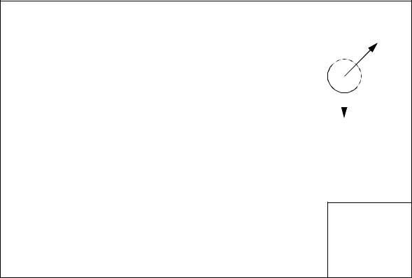
An example calculation including gravitational acceleration is shown in Figure 2.8. The 5kg mass is pulled by two forces, gravity and the arbitrary force ’F’. These forces are described in vector form, with the positive ’z’ axis pointing upwards. To find the equations of motion the forces are summed. To eliminate the second derivative on the inertia term the equation is integrated twice. The result is a set of three vector equations that describe the x, y and z components of the motion. Notice that the units have been carried through these calculations.

translation - 2.9

Assume we have a mass that is acted upon by gravity and F

M = 5Kg

a second constant force vector. To find the position of

the mass as a function of time we first define the grav-

ity vector and position components for the system.


		0	N		0	m	X( t) =	x( t)
		0			0			x( t)
								y( t)
g =	0		------ =	0		----
	0		Kg	0		s2
	–9.81			–9.81				z( t)

Next, sum the forces and set them equal to inertial resistance.

∑

F = Mg + F = M

d 2

X( t)

----

x( t)

5Kg

---- +

= 5Kg

----

y( t)

–9.81

z( t)

–1

x( t)

---- + 0.2Kg

----

y( t)

–9.81

z( t)

Integrate twice to find the

position components.

vx0

–1

x( t)

---- + 0.2Kg

t +

----

y( t)

–9.81

z( t)

–1

x( t)

y( t)

---- + 0.2Kg

t +

–9.81

z( t)

0.1fxt

+ vx

t + x

x( t)

t2 + v

y( t)

0.1f

t + y

z( t)

–9.81

------------- +

0.1fz t

+ vz

t + z0

fx


F = fy	Fg = Mg


fz

Note: When an engineer solves a problem they will always be looking at the equations and unknowns. In this case there are three equations, and there are 9 constants/givens fx, fy, fz, vx0, vy0, xz0, x0, y0 and z0. There are 4 variables/unknowns x, y, z and t. Therefore with 3 equations and 4 unknowns only one value (4-3) is required to find all of the unknown values.

Figure 2.8 Gravity vector calculations

translation - 2.10

Like gravity, magnetic and electrostatic fields can also apply forces to objects. Magnetic forces are commonly found in motors and other electrical actuators. Electrostatic forces are less common, but may need to be considered for highly charged systems.

Given,

FBD:

g =

–9.81

------

M = 2Kg

Find the acceleration.

ans.

a =	1.5	m
		m
	–7.81	---
	–7.81	s
	0

Figure 2.9 Drill problem: find the acceleration of the FBD

2.2.4 Springs

Springs are typically constructed with elastic materials such as metals and plastics, that will provide an opposing force when deformed. The properties of the spring are determined by the Young’s modulus (E) of the material and the geometry of the spring. A primitive spring is shown in Figure 2.10. In this case the spring is a solid member. The relationship between force and displacement is determined by the basic mechanics of materials relationship. In practice springs are more complex, but the parameters (E, A and L) are combined into a more convenient form. This form is known as Hooke’s Law.

translation - 2.11

		L		F
δ =
		------
		F
		EA
	EA		δ	L

F =		-------		δ
	L
F = Kδ				(Hooke’s law)

Figure 2.10 A solid member as a spring

Hooke’s law does have some limitations that engineers must consider. The basic equation is linear, but as a spring is deformed the material approaches plastic deformation, and the modulus of elasticity will change. In addition the geometry of the object changes, also changing the effective stiffness. Springs are normally assumed to be massless. This allows the inertial effects to be ignored, such as a force propagation delay. In applications with fast rates of change the spring mass may become significant, and they will no longer act as an ideal device.

The cases for tension and compression are shown in Figure 2.11. In the case of compression the spring length has been made shorter than its’ normal length. This requires that a compression force be applied. For tension, both the displacement from neutral and the required force reverse direction. It is advisable when solving problems to assume a spring is either in tension or compression, and then select the displacement and force directions accordingly.

translation - 2.12

∆ x = deformed length ASIDE: a spring has a natural or undeformed length. When at this length it is neither in tension or compression

compression as positive:

∆ x

Fc = Ks∆ x

∆ x

Fc = –Ks∆ x

∆ x

Fc = –Ks∆ x

tension as positive:

Ft = Ks∆ x

∆

Ft = –Ks∆ x

∆

Ft = –Ks∆ x

∆ x

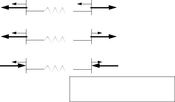
NOTE: the symbols for springs, resistors and inductors are quite often the same or similar. You will need to remember this when dealing with complex systems - and especially in this book where we deal with both types of components.

Figure 2.11 Sign conventions for spring forces and displacements

Previous examples have shown springs with displacements at one end only. In Figure 2.12, springs are shown that have movement at both ends. In these cases the sign of the force applied to the spring is selected with reference to the assumed compression or tension. The primary difference is that care is required to correctly construct the expressions for the tension or compression forces. In all cases the forces on the springs must be assumed and drawn as either tensile or compressive. In the first example the displacement and forces are tensile. The displacement at the left is tensile, so it will be positive, but on the right hand side the displacement is compressive so it is negative. In the second exam-

translation - 2.13

ple the force and both displacements are shown as tensile, so the terms are both positive. In the third example the force is shown as compressive, while the displacements are both shown as tensile, so both terms are negative.

∆ x	1	Ks
F		Ks
∆ x	1	Ks
F		Ks
∆ x	1	Ks
F		Ks

∆ x2		F
		F
		F = Ks( ∆ x1 – ∆ x2)
	∆ x2	F	( ∆ x1 + ∆ x2)
		F
		F = Ks

∆ x2 F	( – ∆ x1 – ∆ x2)
F = Ks

Aside: it is useful to assume that the spring is either in tension or compression, and then make all decisions based on that assumption.

Figure 2.12 Examples of forces when both sides of a spring can move

The example in Figure 2.13 shows two masses separated by a spring. In the first example the spring is assumed to be in tension. When x1 becomes positive it will put the spring in compression, so it is made negative, however a positive x2 will put the spring in tension, so it remains positive. In the second case the spring is assumed to be in compression and this time x2 will put it in tension so it is made negative.

translation - 2.14

Consider the two masses below separated by a spring.

		Ks
M1	x1		M2
M1			M2
				x2

The system can be reduced to free body diagrams assuming the spring is tension.

Ks( – x1 + x2)

Note: In this example the spring is assumed to be in tension and the signs of the magnitude are made negative for terms that result in compression for positive changes.

The system can be reduced to free body diagrams assuming the spring is in compression.

Ks( x1 – x2)

Figure 2.13 Drawing FBDs with interconnecting springs

Sometimes the true length of a spring is important, and the deformation alone is insufficient. In these cases the deformation can be defined as a deformed and undeformed length, as shown in Figure 2.14.

translation - 2.15

∆ x = l1 – l0

where,

∆ x = deformation

l0 = the length when undeformed l1 = the length when deformed

Figure 2.14 Using the actual spring length

In addition to providing forces, springs may be used as energy storage devices. Figure 2.15 shows the equation for energy stored in a spring.

EP	=	K( ∆ x) 2
		-----------------2

Figure 2.15 Energy stored in a spring

translation - 2.16

Given,

N K = 10---

s m

∆ x = 0.1m

Find F assuming the springs are normally 4m long when unloaded

Aside: it can help to draw a FBD of the pin.

Ks		Ks
		F
		F
		∆ x
		∆ x

	10m

ans. F=2N

Figure 2.16 Drill problem: Deformation of a two spring system

translation - 2.17
Draw the FBDs and the equations of motion for the masses
Ks
F			M2
M1			M2
x1			x2
ans.
··			( Ks) + x2( –Ks) = F
x1( M1) + x1			( Ks) + x2( –Ks) = F
x1( Ks)	··	( –M2) + x2( –Ks) = F
x1( Ks)	+ x2	( –M2) + x2( –Ks) = F

Figure 2.17 Drill problem: Draw the FBDs for the masses

<<< < Предыдущая 1 2 34 / 2174 5 6 7 8 9 10 11 12 13 14 15 16 17 18 19 20 21 22 23 24 25 > Следующая >>>

Соседние файлы в предмете [НЕСОРТИРОВАННОЕ]

#
01.12.2018211.46 Кб7Dokument_Microsoft_Office_Word_8.doc
#
01.12.2018210.94 Кб4Dokument_Microsoft_Office_Word_8.doc
#
25.09.2019109.57 Кб4Dopolnennye_mnoy.doc
#
24.11.2019344.58 Кб2DO_Lektsia_4.doc
#
20.09.2019497.15 Кб3drugaya_rab.doc
#
23.03.20165.61 Mб19Dynamic_System_Modeling_and_Control.pdf
#
11.11.2019749.26 Кб4EGE_obschestvo.rtf
#
11.11.20182.31 Mб7ekonomicheskaya_otsenka_investitsy.docx
#
23.05.2015208.65 Кб12ekonomika_2.docx
#
06.09.2019146.43 Кб2Ekzamenatsionnyy_material_dlya_7_klassa_po_russ...doc
#
02.12.20181.33 Mб14elektrostat.doc