

numerical methods - 4.50
g.Repeat step g. using the first-order approximation method.
h.Use a C program to produce a graph of points for the first 10 seconds.
4.10PRACTICE PROBLEM SOLUTIONS
1.
·
x = v
·
y = u
·
v = – 2v – 3x – 5y + 3
·
u = – u – 6y – 9x + sin t
d
----
dt
2.
y·1 y·2 y·3
v·1
v·2
v·3
|
|
|
|
|
|
|
|
|
|
|
|
|
|
|
|
|
|
x |
|
0 |
0 |
1 |
0 |
|
|
x |
|
0 |
|
||||||
y |
= |
0 |
0 |
0 |
1 |
|
|
y |
+ |
0 |
|
||||||
v |
|
–3 –5 –2 |
0 |
|
|
v |
|
3 |
|
||||||||
u |
|
–9 –6 |
0 |
–1 |
|
u |
|
sin t |
|||||||||
|
|
|
|
|
|
|
|
|
|
|
|
|
|
|
|
|
|
=v1
=v2
=v3
=–2v1 – 3y1 – 4v2 – 5y2 – 6v3 – t – F
= |
–v1 |
– |
13 |
|
|
|
|
|
|
|
|
-------12 |
12-----v3 |
|
|
|
|
|
|
|
|
||
|
–v1 |
|
7 |
|
8 |
|
9 |
|
11 |
|
5 |
= |
-------10 |
– |
10-----y1 |
– |
10-----v2 |
– |
10-----y2 |
– |
10-----y3 |
– |
10----- cos ( 5t) |
|
|
|
|
|
|
|
0 |
0 |
|
0 |
|
|
1 |
0 |
|
0 |
|
|
|
|
|
|
|
|
|
|
|
y1 |
|
|
|
|
|
|
|
y1 |
|
0 |
|
||||||||||||||
|
|
0 |
0 |
|
0 |
|
|
0 |
1 |
|
0 |
|
|
|
|
|||||||||||
|
y2 |
|
|
|
|
|
|
|
y2 |
|
0 |
|
||||||||||||||
|
|
0 |
0 |
|
0 |
|
|
0 |
0 |
|
1 |
|
|
|
|
|||||||||||
|
|
|
|
|
|
|
|
|
0 |
|
||||||||||||||||
d |
y |
3 |
= |
|
–3 |
–5 |
0 |
–2 |
–4 |
–6 |
|
y |
3 |
+ |
|
|||||||||||
|
|
|
|
|
||||||||||||||||||||||
---- |
|
|
|
|
|
|
|
– t – F |
||||||||||||||||||
dt |
v1 |
|
|
|
|
|
|
|
|
1 |
|
|
13 |
|
v1 |
|
|
|||||||||
|
|
|
|
|
|
|
|
|
|
|
|
|
|
|
||||||||||||
|
|
|
|
|
|
0 0 |
0 |
– |
----- |
0 |
– |
----- |
|
|
|
|
|
|
5 0 |
|
||||||
|
v2 |
|
12 |
12 |
|
v2 |
|
|
||||||||||||||||||
|
v3 |
|
7 |
9 |
11 |
– |
1 |
8 |
|
0 |
|
|
v3 |
|
–----- cos t |
|||||||||||
|
|
–----- |
–----- |
–----- |
----- |
–----- |
|
|
|
|
10 |
|
||||||||||||||
|
|
|
|
|
|
|
10 |
10 |
10 |
|
10 |
10 |
|
|
|
|
|
|
|
|
|
|
|
|
||
|
|
|
|
|
|
|
|
|
|
|
|
|
|
|
|
|
|
|
||||||||
|
|
|
|
|
|
|
|
|
|
|
|
|
|
|
|
|
|
|
||||||||
numerical methods - 4.51
3.
x
F
M
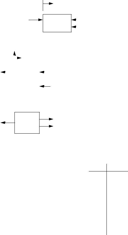
4.
+y
|
|
|
|
+x |
|
Ksx1 |
|
|||
T |
|
|
|
|||||||
|
|
|
|
|
||||||
|
M1 |
|
||||||||
|
|
|
|
|
|
|
|
|
|
|
|
|
|
|
( |
x· |
– x· |
) |
|||
|
|
|
|
|
|
|||||
|
|
|
|
B |
||||||
1 |
1 |
2 |
|
|||||||
B1( x·1 – x·2)
T
M2 |
F |
|
 B2x·2
B2x·2
5.
h = 1
x( t + h) = x( t) + h5( t – 4) 2
|
|
· |
|
· |
|
|
|
|
|
|
|
|
|
|
x = v |
|
|
|
|
|
|
|
|||
|
Kdx |
· |
|
–Kd |
|
–Ks |
|
F |
||||
K |
x |
|||||||||||
|
--------- |
-------- |
---- |
|||||||||
|
s |
|
v = v |
M |
|
+ x |
M |
|
+ |
|
||
|
|
|
|
|
|
|
|
|
M |
|||
|
|
|
|
|
|
|
|
|
|
|
|
|
· |
|
|
|
· |
|
|
|
|
|
·· |
|
|
|
∑F = – T – Ksx1 – B1( x1 – x2) = M1x1 |
|
|
||||||||||||||||||||||||
v1 = x·1 |
|
|
|
|
|
|
|
|
|
|
|
|
|
|
|
|
|
|
|
|
|
|
|
|||
v2 = x·2 |
–Ks |
|
|
|
|
|
–B1 |
|
|
|
|
|
|
|
|
|
|
|||||||||
· |
= x |
|
+ v |
|
|
|
+ v |
|
|
B1 |
|
+ |
|
–T |
||||||||||||
v |
|
|
-------- |
|
|
-------- |
|
|
|
------ |
|
------ |
||||||||||||||
|
1 |
|
1 |
M |
1 |
|
|
|
1 |
M |
1 |
|
|
|
2 |
M |
|
M |
||||||||
|
|
|
|
|
|
|
|
|
|
|
|
|
|
|
|
|
|
|
1 |
|
|
|
1 |
|||
|
|
|
|
|
|
|
|
· |
|
|
|
· |
|
|
|
|
|
|
|
· |
|
|
|
|
·· |
|
∑F = – T + B1( x1 |
– x2) + F – B2x2 |
= M2x2 |
||||||||||||||||||||||||
· |
= v |
|
B1 |
|
+ v |
|
|
–B1 |
– B2 |
+ |
|
– T + F |
||||||||||||||
v |
|
|
------ |
|
2 |
-------------------- |
|
|
----------------- |
|||||||||||||||||
|
2 |
|
1 |
M |
|
|
|
M |
2 |
|
|
|
|
M |
2 |
|
||||||||||
|
|
|
|
2 |
|
|
|
|
|
|
|
|
|
|
|
|
|
|
|
|
|
|
||||
t x
00
180
2125
3145
4150
5150
6155
7175
8220
9300
10425
numerical methods - 4.52
6.
x' = 3 – 0.25x |
|
|
|
x( t + h) |
= x( t) + h |
d |
|
----x( t) |
|
||
|
|
dt |
|
x( t + h) |
= x( t) + 1( 3 – 0.25x( t) ) |
||
x( t + h) |
= 0.75x( t) + 3 |
|
|
t |
x |
x’ |
|
|
|
0 |
1 |
2.75 |
1 |
3.75 |
2.06 |
2 |
5.81 |
1.55 |
3 |
7.36 |
1.16 |
4 |
8.52 |
0.870 |
5 |
9.39 |
0.652 |
6 |
10.0 |
0.489 |
7 |
10.5 |
0.367 |
8 |
10.9 |
0.275 |
9 |
11.2 |
0.206 |
10 |
11.4 |
|
|
|
|
numerical methods - 4.53
7.
//integrate.sce - A simple program to integrate a function
//To run this in Scilab use 'File' then 'Exec'.
//by: H. Jack Sept., 9, 2002
//define the function
function foo=f(x)
foo = 5 * x + 2 * log(sin(x) / x); endfunction
//Set the time length and step size steps = 10;
x_start = 1; x_end = 1.2;
x_delta = (x_end - x_start) / steps;
//Loop for rectangular integration
total = 0; // set the initial sum to zero for i=0:steps,
x = x_start + i * x_delta; total = total + f(x);
end
total = total * x_delta;
printf("Rectangular integration value %f\n", total); // Loop for trapezoidal integration
total = 0; // set the initial sum to zero for i=0:steps,
x = x_start + i * x_delta; if i == 0 then
total = total + f(x); elseif i == steps then
total = total + f(x);
else
total = total + 2 * f(x);
end
end
total = total * x_delta / 2;
printf("Trapezoidal integration value %f\n", total); // Loop for Simpson's rule integration
total = 0; // set the initial sum to zero even = 0;
for i=0:steps,
x = x_start + i * x_delta; if i == 0 then
total = total + f(x); elseif i == steps then
total = total + f(x);
else
even = even + 1; if even > 1 then
total = total + 4 * f(x); even = 0;
else
total = total + 2 * f(x);
end
end
end
total = total * x_delta / 3;
printf("Simpsons rule integration value %f\n", total);
numerical methods - 4.54
8.
#include <stdio.h>
steps = 100, i;
double theta, omega, step_t, theta_last, omega_last;
theta = 0.0; omega = 0.0; step_t = 1.0;
for(i = 0; i < steps; i++){ theta_last = theta; omega_last = omega;
theta = theta_last + step_t * omega_last;
omega = omega_last + step_t*(-3 * omega_last - 9 * theta_last + 10); printf("%f %f %f \n", i+step_t, theta, omega);
}
}
numerical methods - 4.55
9.
a) |
Vo( t) = – 8.331e–0.6t cos ( 1.960t – 0.238) + 8.095 |
||
b) |
· |
|
|
Vo = Yo |
|
||
|
Y·o |
= – 1.2Yo – 4.2Vo + 34 |
|
|
// assign4_1.sce |
||
|
// by: H. Jack Sept., 23, 2003 |
||
|
v0 |
= 0; |
// initial conditions |
|
y0 |
= 1; |
|
X=[v0, y0];
//define the state matrix function
//the values returned are [x, v] function foo=f(state,t)
foo = [ state($, 2), -1.2*state($,2) - 4.2*state($,1) + 34]; endfunction
//Set the time length and step size for the integration
steps = 1000; t_start = 0; t_end = 10;
h = (t_end - t_start) / steps; t = [t_start];
//
// Loop for integration
//
for i=1:steps,
t = [t ; t($,:) + h];
F1 = h * f(X($,:), t($,:));
F2 = h * f(X($,:) + F1/2.0, t($,:) + h/2.0);
F3 = h * f(X($,:) + F2/2.0, t($,:) + h/2.0);
F4 = h * f(X($,:) + F3, t($,:) + h);
X = [X ; X($,:) + (F1 + 2.0*F2 + 2.0*F3 + F4)/6.0];
end
//
// Graph the values
//
plot2d(t, X, [-2, -5], leg="position@velocity"); xtitle('Time (s)');
//
// Generate points from the given function
//
XX = [v0];
for i=1:steps,
tt = i * h;
XX = [XX ; -8.331 * exp(-0.6 * tt) * cos( 1.960 * tt - 0.238) + 8.095];
end
plot2d(t, XX, [-4], leg="explicit");
c) The two curves produced by the scilab program overlap, so the results agree.
numerical methods - 4.56
10.
|
|
|
|
|
|
|
|
|
|
|
|
· |
|
|
|
|
|
|
|
|
|
|
|
|
|
|
|
|
|
|
|
|
|
|
|
|
|
|
|
|
|
F |
|
|
|
|
|
|
|
Kdx |
|
|
|
|
|
|
|
|
|
|
|
|
|
|
|
|
|
|
· |
|
|
|
|
|
·· |
|
|
|
|||||
|
|
|
|
|
|
|
|
|
|
|
|
|
|
|
|
|
|
|
|
|
|
|
|
|
|
|
|
|
|
|
|
|
|||||||||
|
|
|
|
|
|
|
|
|
|
|
|
|
|
|
|
|
|
|
|
|
|
|
∑F = F – Kdx – Ksx = Mx |
|
|
|
|||||||||||||||
|
|
|
M |
|
|
|
|
|
Ksx |
|
|
|
|
|
|
|
|
|
|
|
|
|
|||||||||||||||||||
|
|
|
|
|
|
|
|
|
|
|
|
|
|
|
|
|
|
|
|
|
|||||||||||||||||||||
|
|
|
|
|
|
|
|
|
|
|
|
|
|
|
|
|
|
|
·· |
|
|
|
|
· |
|
|
|
|
|
|
|
|
|
|
|
||||||
|
|
|
|
|
|
|
|
|
|
|
|
|
|
|
|
|
|
|
|
|
|
|
Mx + Kdx + Ksx = F |
|
|
|
|
|
|
||||||||||||
|
|
|
|
|
|
|
|
|
|
|
|
|
|
|
|
|
|
|
|
|
|
|
|
|
|
|
|
|
|||||||||||||
|
|
|
|
|
|
|
|
|
|
|
|
x |
|
|
|
|
|
|
|
|
|
|
·· |
|
|
|
|
|
· |
|
|
|
|
|
|
|
|
|
|
|
|
|
|
|
|
|
|
|
|
|
|
|
|
|
|
|
|
|
|
|
|
|
|
|
|
|
|
|
|
|
|
|
|
|
|
|
|
|
|
||||
|
|
|
|
|
|
|
|
|
|
|
|
|
|
|
|
|
|
|
|
|
10x + 10x + 10x |
= 10 |
|
|
|
|
|
||||||||||||||
|
|
|
|
|
|
|
|
|
|
|
|
|
|
|
|
|
|
|
|
|
|
|
|
|
|
||||||||||||||||
|
|
|
|
|
|
|
|
|
|
|
|
|
|
|
|
|
|
|
|
|
|
|
·· |
|
· |
|
|
|
|
= 1 |
|
|
|
|
|
|
|
|
|
|
|
|
|
|
|
|
|
|
|
|
|
|
|
|
|
|
|
|
|
|
|
|
|
|
|
|
|
|
|
|
|
|
|
|
|
|
|
|
|
||||
homogeneous: |
|
|
|
|
|
|
|
|
|
|
|
|
|
|
|
|
|
|
x + x + x |
|
|
|
|
|
|
|
|
|
|
||||||||||||
·· |
|
|
|
· |
|
|
|
= 0 |
|
|
|
|
|
|
|
|
|
|
|
|
|
|
|
|
|
|
|
|
|
|
|||||||||||
|
|
|
|
|
x + x + x |
|
|
|
|
|
|
|
|
|
|
|
|
|
|
|
|
|
|
|
|
|
|
||||||||||||||
|
|
|
|
A2 + A + 1 = 0 |
|
|
|
|
|
|
|
|
|
|
|
|
|
|
|
|
|
|
|
|
|
|
|||||||||||||||
|
|
|
|
A |
= |
– 1 ± 1 – 4( 1) ( 1) |
|
= |
– |
0.5 ± |
|
3 |
|
|
|
|
|
|
|
||||||||||||||||||||||
|
|
|
|
--------------------------------------------- |
|
|
j------ |
|
|
|
|
|
|
|
|||||||||||||||||||||||||||
|
|
|
|
|
|
|
|
|
|
|
|
|
|
|
|
|
|
2 |
( 1) |
|
|
|
|
|
|
|
|
|
|
|
2 |
|
|
|
|
|
|
|
|||
|
|
|
|
x |
|
|
= |
C |
|
e |
–0.5t |
cos |
3 |
|
+ |
|
C |
|
|
|
|
|
|
|
|
|
|
|
|
|
|||||||||||
|
|
|
|
|
|
1 |
|
|
|
------t |
|
|
|
|
|
|
|
|
|
|
|
|
|
|
|||||||||||||||||
|
|
|
|
|
|
|
h |
|
|
|
|
|
|
|
|
|
|
|
|
|
2 |
|
|
|
|
2 |
|
|
|
|
|
|
|
|
|
|
|
||||
particular: |
|
xp |
|
= B |
|
|
|
|
|
|
|
|
|
|
|
|
|
|
|
|
|
|
|
|
|
|
|
|
|
|
|
|
|||||||||
|
|
|
|
|
|
|
|
|
|
|
|
|
|
|
|
|
|
|
|
|
|
|
|
|
|
|
|
|
|
|
|
|
|||||||||
|
|
|
|
0 + 0 + B = 1 |
|
|
|
|
|
|
|
|
|
|
|
|
|
|
|
|
|
|
|
|
|
|
|
||||||||||||||
|
|
|
|
xp |
= 1 |
|
|
|
|
|
|
|
|
|
|
|
|
|
|
|
|
|
|
|
|
|
|
|
|
|
|
|
|
|
|||||||
initial conditions: |
|
|
|
|
|
|
|
|
|
|
|
|
|
|
|
|
|
|
|
|
|
|
|
|
|
|
|
|
|
|
|
|
|
||||||||
|
|
|
x = |
x |
|
+ x |
|
= |
C |
|
|
e |
–0.5t |
cos |
3 |
|
+ 1 |
|
|
|
|
|
|||||||||||||||||||
|
|
|
h |
p |
1 |
|
|
------t + C |
|
|
|
|
|
||||||||||||||||||||||||||||
|
|
|
|
|
|
|
|
|
|
|
|
|
|
|
|
|
|
|
|
|
|
|
|
|
2 |
|
|
2 |
|
|
|
|
|
|
|
|
|||||
|
|
|
x' |
|
|
= |
|
|
3 |
|
|
|
–0.5t |
sin |
|
3 |
|
|
|
C |
– 0.5C |
|
e |
–0.5t |
cos |
|
3 |
|
|||||||||||||
|
|
|
|
|
–------C e |
|
|
|
------t + |
|
|
|
|
------t + C |
|||||||||||||||||||||||||||
|
|
|
|
|
|
|
|
|
|
|
|
2 |
|
|
1 |
|
|
|
|
|
|
2 |
|
|
|
|
2 |
|
|
1 |
|
|
|
|
|
2 |
2 |
||||
|
|
|
|
x'( 0) |
|
= |
|
|
|
3 |
|
|
|
|
|
( C2) |
– 0.5C1 cos ( C2) |
|
= |
0 |
|
|
|
||||||||||||||||||
|
|
|
|
|
–------C sin |
|
|
|
|
||||||||||||||||||||||||||||||||
|
|
|
|
|
|
|
|
|
3 |
|
|
|
|
|
2 |
|
1 |
|
|
|
|
|
|
|
|
|
|
|
|
|
|
|
|
|
|
|
|
|
|
||
|
|
|
|
– |
|
|
|
|
|
|
|
|
|
|
|
|
|
|
|
|
|
|
|
|
|
|
|
|
|
|
|
|
|
|
|
|
|
|
|
||
|
|
|
|
------ sin ( C ) = 0.5 cos ( C ) |
|
|
|
|
|
|
|
|
|
|
|
|
|
||||||||||||||||||||||||
|
|
|
|
|
|
|
2 |
|
|
|
|
|
2 |
|
|
|
|
|
|
|
|
|
|
2 |
|
|
|
|
|
|
|
|
|
|
|
|
|
||||
|
|
|
|
tan ( C ) |
|
|
|
–1 |
|
|
|
|
|
|
|
C |
|
|
= |
atan |
|
–1 |
|
= |
–0.5236 |
|
|||||||||||||||
|
|
|
|
= ------ |
|
|
|
|
|
|
|
|
|
------ |
|
|
|||||||||||||||||||||||||
|
|
|
|
|
|
|
|
|
|
|
|
2 |
|
|
|
|
|
3 |
|
|
|
|
|
|
|
|
2 |
|
|
|
3 |
|
|
|
|
|
|
||||
|
|
|
|
|
|
|
|
|
|
|
|
|
|
|
|
|
|
|
|
|
|
|
|
|
|
|
|
|
|
|
|
|
|
|
|
|
|
|
|
||
|
|
|
|
x( 0) |
|
= C1 cos ( –0.5236) + 1 = 0 |
|
|
|
|
|
|
|
|
|
|
|||||||||||||||||||||||||
|
|
|
|
C |
|
|
|
= |
|
|
|
|
|
–1 |
|
|
|
|
|
= |
|
–1.155 |
|
|
|
|
|
|
|
|
|
|
|||||||||
|
|
|
|
|
|
|
-------------------------------- |
|
|
|
|
|
|
|
|
|
|
|
|||||||||||||||||||||||
|
|
|
|
|
|
1 |
|
|
|
cos ( –0.5236) |
|
|
|
|
|
|
|
|
|
|
|
|
|
|
|
|
|
|
|||||||||||||
|
|
|
|
|
|
|
|
|
|
|
|
|
|
|
|
|
|
|
|
|
|
|
|
|
|
|
|
|
|
|
|
|
|
|
|
||||||
x = –1.155e |
–0.5t |
sin |
|
|
|
3 |
|
|
|
|
|
|
|
+ 1 |
|
|
|
|
|
|
|
|
|
|
|
|
|
||||||||||||||
|
|
|
|
|
|
|
------t + 1.047 |
|
|
|
|
|
|
|
|
|
|
|
|
|
|||||||||||||||||||||
|
|
|
|
|
|
|
|
|
|
|
|
|
|
|
2 |
|
|
|
|
|
|
|
|
|
|
|
|
|
|
|
|
|
|
|
|
|
|
|
|
||
First peak is at x=1.219, t=3.63s on graph

numerical methods - 4.57
11.
a) |
·· |
|
|
Kd |
· |
|
|
|
Ks |
x = |
F |
|
|
|
|
|
|
|
|
|
|
|
|
|
|
|
|
||||||||
x + |
----- |
x + |
----- |
|
---- |
|
|
|
|
|
|
|
|
|
|
|
|
|
|
|
|||||||||||||||
|
|
|
|
|
|
M |
|
N |
M |
|
|
|
M |
|
|
|
|
|
|
|
–5t |
|
|
|
|
|
|||||||||
b) |
Kd |
= |
100 |
|
|
|
x1 |
( t) |
= |
– 0.115e |
cos ( 5 |
|
3t – 0.524) + 0.10 |
||||||||||||||||||||||
--- |
|
|
|
|
|
|
|||||||||||||||||||||||||||||
|
|
|
|
|
|
|
|
|
|
m |
N |
|
|
|
|
|
|
|
|
|
|
|
|
|
|
–0.1t |
|
|
–5 |
|
–999.9t |
|
|||
|
Kd |
= |
|
10000 |
|
|
x1 |
( t) |
= – 0.1e |
+ 10 |
e |
+ 0.10 |
|||||||||||||||||||||||
|
|
--- |
|
|
|
|
|
|
|||||||||||||||||||||||||||
|
|
|
|
|
|
|
|
|
|
|
|
|
m |
|
|
|
|
|
|
|
|
|
|
|
|
|
|
|
|
|
|
|
|
|
|
c) |
|
|
|
|
|
|
|
|
|
|
|
|
0 |
|
1 |
|
|
|
|
|
|
|
|
|
|
|
|
|
|
|
|
|
|
|
|
d |
|
X |
0 |
|
|
|
|
|
|
|
|
X |
0 |
|
|
0 |
|
|
|
|
|
|
|
|
|
|
|||||||||
|
|
|
|
|
|
|
|
|
|
|
|
|
|
|
|
|
|
|
|
|
|
||||||||||||||
|
|
|
|
|
|
|
|
|
|
|
|
|
|
|
|
|
|
|
|
|
|
|
|
|
|
||||||||||
|
---- |
|
|
|
= |
|
–Ks |
–Kd |
|
|
|
+ |
|
|
F |
|
|
|
|
|
|
|
|
|
|||||||||||
|
dt |
|
X1 |
|
|
|
-------- |
--------- |
|
X1 |
|
|
---- |
|
|
|
|
|
|
|
|
|
|||||||||||||
|
|
|
|
|
|
|
|
|
|
|
|
|
M |
|
M |
|
|
|
|
|
|
|
M |
|
|
|
|
|
|
|
|
|
|||
|
|
|
|
|
|
|
|
|
|
|
|
|
|
|
|
|
|
|
|
|
|
|
|
|
|
|
|||||||||
|
|
|
|
|
|
|
|
|
|
|
|
|
|
|
|
|
|
|
|
|
|
|
|
|
|
|
|
|
|
|
|
|
|
|
|
g)For 100N/m: all solutions are underdamped and overshoot at; b) 0.1163 at t = 0.363s
d)0.1166 at t = 0.361s
e)0.1163 at t = 0.363s
f)0.1163 at t = 0.360s
For 10000N/m: all solutions are overdamped. The time to reach the time constant (at 0.06321) is,
b) 0.06321 at t = 10.001s
d)0.06321 at t = 10.000s
e)0.06321 at t = 10.000s
f)0.06321 at t = 10.0s
h) |
K |
|
= 200 |
Ns |
(verify with numerical integration also) |
d |
------ |
||||
|
|
|
m |
|
numerical methods - 4.58
12.
b)x·1 = v1
· |
= |
|
x |
|
|
–Ks1 |
+ x |
|
Ks1 |
|
+ |
F |
|
|
|
|
|
|
|
|
||||||||||||||||
x |
|
|
|
|
----------- |
|
|
------- |
|
|
------ |
|
|
|
|
|
|
|
|
|
||||||||||||||||
|
1 |
|
|
|
|
|
1 |
M |
1 |
|
|
|
|
|
2 |
M |
1 |
|
|
|
M |
|
|
|
|
|
|
|
|
|||||||
x·2 = v2 |
|
|
|
|
|
|
|
|
|
|
|
|
|
|
|
1 |
|
|
|
|
|
|
|
|
|
|||||||||||
|
|
|
|
|
|
|
|
|
|
|
|
|
|
|
|
|
|
|
|
|
|
|
|
|
|
|
|
|
||||||||
· |
= |
|
x |
|
Ks1 |
+ |
x |
|
|
– Ks1 |
|
– Ks2 |
|
|
|
|
|
|
|
|
||||||||||||||||
x |
|
|
|
|
------- |
|
|
-------------------------- |
|
|
|
|
|
|
|
|
|
|
||||||||||||||||||
|
1 |
|
|
|
|
|
1 |
M |
2 |
|
|
|
|
2 |
|
M |
2 |
|
|
|
|
|
|
|
|
|
||||||||||
|
|
|
|
|
|
|
|
|
|
|
|
|
|
|
|
|
|
|
|
|
|
|
|
|
|
|
|
|
|
|
|
|
|
|||
c) |
|
|
|
|
|
|
|
|
|
|
|
|
|
|
|
|
|
|
|
|
|
|
|
|
|
|
|
|
|
|
|
|
|
|
|
|
|
|
|
|
|
|
|
|
|
|
|
|
0 |
|
1 |
|
|
|
0 |
|
|
0 |
|
|
|
|
|
|
|
|
|
||||||
|
|
|
|
|
|
|
|
|
|
|
|
|
|
|
|
|
|
|
|
|
|
|
|
|
|
|
|
|||||||||
|
|
x1 |
|
|
|
|
–Ks1 |
0 |
|
|
Ks1 |
0 |
|
x1 |
|
0 |
|
|||||||||||||||||||
d |
v |
|
|
|
|
|
|
----------- |
|
|
------- |
|
v |
|
|
|
|
F |
||||||||||||||||||
1 |
|
|
|
|
|
M |
1 |
|
|
|
|
|
M |
1 |
|
|
|
1 |
|
------ |
||||||||||||||||
---- |
x |
|
= |
|
|
|
|
|
|
0 |
|
|
|
|
|
1 |
|
x |
+ |
M1 |
||||||||||||||||
dt |
2 |
|
|
|
|
|
|
|
0 |
|
|
|
|
0 |
|
|
|
2 |
|
0 |
|
|||||||||||||||
|
|
|
|
|
|
|
|
|
|
|
|
|
|
|
|
|
|
|
|
|
|
|
|
|
|
|
|
|
|
|
||||||
|
|
v |
|
|
|
|
|
|
|
Ks1 |
|
|
|
|
– Ks1 |
– Ks2 |
|
v |
|
|
|
|
||||||||||||||
|
|
2 |
|
|
|
|
|
|
|
|
|
|
2 |
|
0 |
|
||||||||||||||||||||
|
|
|
|
|
|
|
|
|
------- |
|
0 |
|
-------------------------- 0 |
|
|
|
|
|
||||||||||||||||||
|
|
|
|
|
|
|
|
|
|
|
M2 |
|
|
|
|
|
M2 |
|
|
|
|
|
|
|
|
|
|
|
||||||||
|
|
|
|
|
|
|
|
|
|
|
|
|
|
|
|
|
|
|
|
|
|
|
|
|
|
|
||||||||||
numerical methods - 4.59
// System component values Ks1 = 100;
Ks2 = 100;
e), f), g) M1 = 1;
M2 = 1;
F = 1;
x0 = 0; // initial conditions
v0 = 0;
x1 = 0;
v1 = 0;
X=[x0, v0, x1, v1];
//define the state matrix function the values returned are [x, v] function foo=f(state,t)
foo = [ state($,2), -Ks1/M1*state($,1)+Ks1/M1*state($,3)+F/M1, state($,4), Ks1/M2*state($,1)-(Ks1+Ks2)/M2*state($,3)];
endfunction
//Set the time length and step size for the integration
steps = 10000; t_start = 0; t_end = 10;
h = (t_end - t_start) / steps; t = [t_start];
//Loop for integration for i=1:steps,
t = [t ; t($,:) + h];
F1 = h * f(X($,:), t($,:));
F2 = h * f(X($,:) + F1/2.0, t($,:) + h/2.0); F3 = h * f(X($,:) + F2/2.0, t($,:) + h/2.0); F4 = h * f(X($,:) + F3, t($,:) + h);
X = [X ; X($,:) + (F1 + 2.0*F2 + 2.0*F3 + F4)/6.0];
end
//Graph the values for part e)
plot2d(t, X, [-2, -5, -7, -9], leg="position1@velocity1@position2@velocity2"); xtitle('Time (s)');
// printf the values for part f) printf("\n\nPart e output\n\n"); for time_count=0:20,
i = (time_count/2) / h + 1;
printf("Point at t=%f x1=%f, v1=%f, x2=%f, v2=%f \n", time_count/2, X(i, 1), X(i, 2), X(i, 3), X(i, 4));
end
// First order integration for part h) X=[x0, v0, x1, v1];
t = [t_start]; for i=1:steps,
t = [t ; t($,:) + h];
F1 = h * f(X($,:), t($,:));
X = [X ; X($,:) + F1 ];
end
printf("\n\nPart g output \n\n"); for time_count=0:20,
i = (time_count/2) / h + 1;
printf("Point at t=%f x1=%f, v1=%f, x2=%f, v2=%f \n", time_count/2, X(i, 1), X(i, 2), X(i, 3), X(i, 4));
end