

principles_of_economics_gregory_mankiw
.pdfCHAPTER 6 |
SUPPLY, DEMAND, AND GOVERNMENT POLICIES |
125 |
(a) A Price Floor That Is Not Binding |
(b) A Price Floor That Is Binding |
|
Price of |
|
|
Price of |
|
|
|
Ice-Cream |
|
Supply |
Ice-Cream |
|
Supply |
|
Cone |
|
Cone |
|
|||
|
|
|
|
|
||
Equilibrium |
|
|
|
Surplus |
|
|
|
|
|
|
|
|
|
price |
|
|
$4 |
|
|
Price |
|
|
|
|
|
|
|
$3 |
|
|
3 |
|
|
floor |
|
Price |
|
|
|
||
|
|
|
|
|
|
|
2 |
|
floor |
Equilibrium |
|
|
|
|
|
|
|
|
||
|
|
|
price |
|
|
|
|
|
Demand |
|
|
|
Demand |
0 |
100 |
Quantity of |
0 |
80 |
120 |
Quantity of |
|
Equilibrium |
Ice-Cream |
|
Quantity |
Quantity |
Ice-Cream |
|
quantity |
Cones |
|
demanded |
supplied |
Cones |
|
|
|
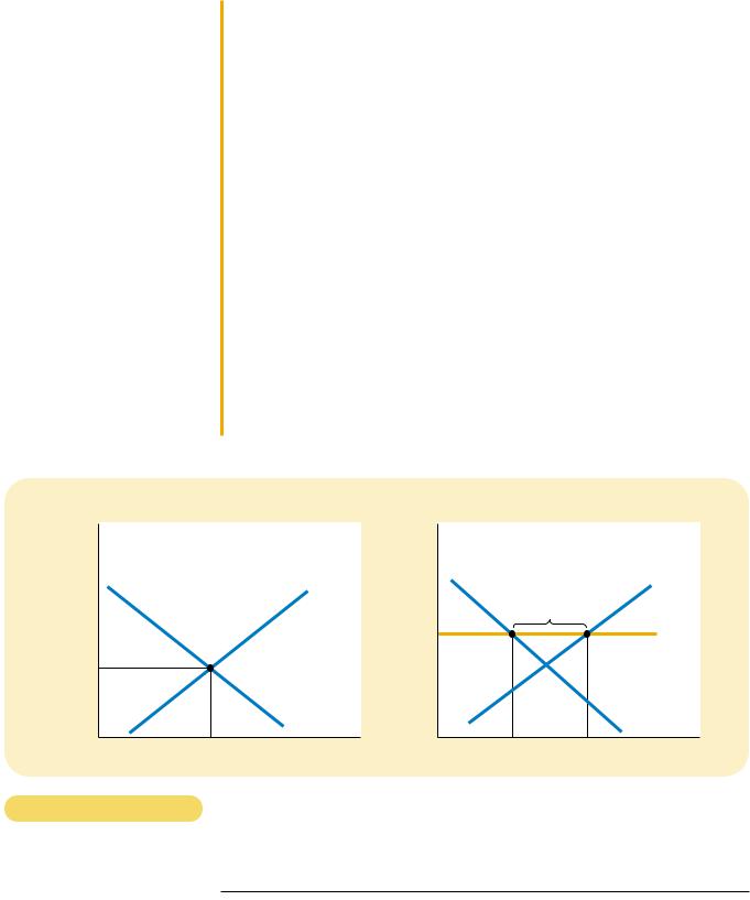
A MARKET WITH A PRICE FLOOR. In panel (a), the government imposes a price floor of |
Figur e 6-4 |
|
$2. Because this is below the equilibrium price of $3, the price floor has no effect. The |
|
|
|
|
|
market price adjusts to balance supply and demand. At the equilibrium, quantity supplied |
|
|
and quantity demanded both equal 100 cones. In panel (b), the government imposes a |
|
|
price floor of $4, which is above the equilibrium price of $3. Therefore, the market price |
|
|
equals $4. Because 120 cones are supplied at this price and only 80 are demanded, there is |
|
|
a surplus of 40 cones. |
|
|
|
|
|
|
|
|
When the government imposes a price floor on the ice-cream market, two outcomes are possible. If the government imposes a price floor of $2 per cone when the equilibrium price is $3, we obtain the outcome in panel (a) of Figure 6-4. In this case, because the equilibrium price is above the floor, the price floor is not binding. Market forces naturally move the economy to the equilibrium, and the price floor has no effect.
Panel (b) of Figure 6-4 shows what happens when the government imposes a price floor of $4 per cone. In this case, because the equilibrium price of $3 is below the floor, the price floor is a binding constraint on the market. The forces of supply and demand tend to move the price toward the equilibrium price, but when the market price hits the floor, it can fall no further. The market price equals the price floor. At this floor, the quantity of ice cream supplied (120 cones) exceeds the quantity demanded (80 cones). Some people who want to sell ice cream at the going price are unable to. Thus, a binding price floor causes a surplus.
Just as price ceilings and shortages can lead to undesirable rationing mechanisms, so can price floors and surpluses. In the case of a price floor, some sellers are unable to sell all they want at the market price. The sellers who appeal to the personal biases of the buyers, perhaps due to racial or familial ties, are better able to sell their goods than those who do not. By contrast, in a free market, the price serves as the rationing mechanism, and sellers can sell all they want at the equilibrium price.
126 |
PART TWO SUPPLY AND DEMAND I: HOW MARKETS WORK |
CASE STUDY THE MINIMUM WAGE
An important example of a price floor is the minimum wage. Minimum-wage laws dictate the lowest price for labor that any employer may pay. The U.S. Congress first instituted a minimum wage with the Fair Labor Standards Act of 1938 to ensure workers a minimally adequate standard of living. In 1999 the minimum wage according to federal law was $5.15 per hour, and some state laws imposed higher minimum wages.
To examine the effects of a minimum wage, we must consider the market for labor. Panel (a) of Figure 6-5 shows the labor market which, like all markets, is subject to the forces of supply and demand. Workers determine the supply of labor, and firms determine the demand. If the government doesn’t intervene, the wage normally adjusts to balance labor supply and labor demand.
Panel (b) of Figure 6-5 shows the labor market with a minimum wage. If the minimum wage is above the equilibrium level, as it is here, the quantity of labor supplied exceeds the quantity demanded. The result is unemployment. Thus, the minimum wage raises the incomes of those workers who have jobs, but it lowers the incomes of those workers who cannot find jobs.
To fully understand the minimum wage, keep in mind that the economy contains not a single labor market, but many labor markets for different types of workers. The impact of the minimum wage depends on the skill and experience of the worker. Workers with high skills and much experience are not affected, because their equilibrium wages are well above the minimum. For these workers, the minimum wage is not binding.
(a) A Free Labor Market
Wage |
|
|
|
|
Labor |
|
|
supply |
Equilibrium |
|
|
wage |
|
|
|
|
Labor |
|
|
demand |
0 |
Equilibrium |
Quantity of |
|
employment |
Labor |
(b) A Labor Market with a Binding Minimum Wage
Wage |
|
|
|
|
|
|
Labor |
|
Labor surplus |
supply |
|
|
|
||
Minimum |
(unemployment) |
|
|
|
|
|
|
wage |
|
|
|
|
|
|
Labor |
|
|
|
demand |
0 |
Quantity |
Quantity |
Quantity of |
|
demanded |
supplied |
Labor |
Figur e 6-5
HOW THE MINIMUM WAGE AFFECTS THE LABOR MARKET. Panel (a) shows a labor
market in which the wage adjusts to balance labor supply and labor demand. Panel (b) shows the impact of a binding minimum wage. Because the minimum wage is a price floor, it causes a surplus: The quantity of labor supplied exceeds the quantity demanded. The result is unemployment.

CHAPTER 6 SUPPLY, DEMAND, AND GOVERNMENT POLICIES |
127 |
The minimum wage has its greatest impact on the market for teenage labor. The equilibrium wages of teenagers are low because teenagers are among the least skilled and least experienced members of the labor force. In addition, teenagers are often willing to accept a lower wage in exchange for on-the-job training. (Some teenagers are willing to work as “interns” for no pay at all. Because internships pay nothing, however, the minimum wage does not apply to them. If it did, these jobs might not exist.) As a result, the minimum wage is more often binding for teenagers than for other members of the labor force.
Many economists have studied how minimum-wage laws affect the teenage labor market. These researchers compare the changes in the minimum wage over time with the changes in teenage employment. Although there is some debate about how much the minimum wage affects employment, the typical study finds that a 10 percent increase in the minimum wage depresses teenage employment between 1 and 3 percent. In interpreting this estimate, note that a 10 percent increase in the minimum wage does not raise the average wage of teenagers by 10 percent. A change in the law does not directly affect those teenagers who are already paid well above the minimum, and enforcement of minimum-wage laws is not perfect. Thus, the estimated drop in employment of 1 to 3 percent is significant.
In addition to altering the quantity of labor demanded, the minimum wage also alters the quantity supplied. Because the minimum wage raises the wage that teenagers can earn, it increases the number of teenagers who choose to look for jobs. Studies have found that a higher minimum wage influences which teenagers are employed. When the minimum wage rises, some teenagers who are still attending school choose to drop out and take jobs. These new dropouts displace other teenagers who had already dropped out of school and who now become unemployed.
The minimum wage is a frequent topic of political debate. Advocates of the minimum wage view the policy as one way to raise the income of the working poor. They correctly point out that workers who earn the minimum wage can afford only a meager standard of living. In 1999, for instance, when the minimum wage was $5.15 per hour, two adults working 40 hours a week for every week of the year at minimum-wage jobs had a total annual income of only $21,424, which was less than half of the median family income. Many advocates of the minimum wage admit that it has some adverse effects, including unemployment, but they believe that these effects are small and that, all things considered, a higher minimum wage makes the poor better off.
Opponents of the minimum wage contend that it is not the best way to combat poverty. They note that a high minimum wage causes unemployment, encourages teenagers to drop out of school, and prevents some unskilled workers from getting the on-the-job training they need. Moreover, opponents of the minimum wage point out that the minimum wage is a poorly targeted policy. Not all minimum-wage workers are heads of households trying to help their families escape poverty. In fact, fewer than a third of minimum-wage earners are in families with incomes below the poverty line. Many are teenagers from middle-class homes working at part-time jobs for extra spending money.
EVALUATING PRICE CONTROLS
One of the Ten Principles of Economics discussed in Chapter 1 is that markets are usually a good way to organize economic activity. This principle explains why

128 |
PART TWO SUPPLY AND DEMAND I: HOW MARKETS WORK |
economists usually oppose price ceilings and price floors. To economists, prices are not the outcome of some haphazard process. Prices, they contend, are the result of the millions of business and consumer decisions that lie behind the supply and demand curves. Prices have the crucial job of balancing supply and demand and, thereby, coordinating economic activity. When policymakers set prices by legal decree, they obscure the signals that normally guide the allocation of society’s resources.
Another one of the Ten Principles of Economics is that governments can sometimes improve market outcomes. Indeed, policymakers are led to control prices because they view the market’s outcome as unfair. Price controls are often aimed at helping the poor. For instance, rent-control laws try to make housing affordable for everyone, and minimum-wage laws try to help people escape poverty.
Yet price controls often hurt those they are trying to help. Rent control may keep rents low, but it also discourages landlords from maintaining their buildings and makes housing hard to find. Minimum-wage laws may raise the incomes of some workers, but they also cause other workers to be unemployed.
Helping those in need can be accomplished in ways other than controlling prices. For instance, the government can make housing more affordable by paying a fraction of the rent for poor families. Unlike rent control, such rent subsidies do not reduce the quantity of housing supplied and, therefore, do not lead to housing shortages. Similarly, wage subsidies raise the living standards of the working poor without discouraging firms from hiring them. An example of a wage subsidy is the earned income tax credit, a government program that supplements the incomes of low-wage workers.
Although these alternative policies are often better than price controls, they are not perfect. Rent and wage subsidies cost the government money and, therefore, require higher taxes. As we see in the next section, taxation has costs of its own.
QUICK QUIZ: Define price ceiling and price floor, and give an example of each. Which leads to a shortage? Which leads to a surplus? Why?
TAXES
All governments—from the federal government in Washington, D.C., to the local governments in small towns—use taxes to raise revenue for public projects, such as roads, schools, and national defense. Because taxes are such an important policy instrument, and because they affect our lives in many ways, the study of taxes is a topic to which we return several times throughout this book. In this section we begin our study of how taxes affect the economy.
To set the stage for our analysis, imagine that a local government decides to hold an annual ice-cream celebration—with a parade, fireworks, and speeches by town officials. To raise revenue to pay for the event, it decides to place a $0.50 tax on the sale of ice-cream cones. When the plan is announced, our two lobbying groups swing into action. The National Organization of Ice Cream Makers claims that its members are struggling to survive in a competitive market, and it argues that buyers of ice cream should have to pay the tax. The American Association of Ice Cream Eaters claims that consumers of ice cream are having trouble making ends meet, and it argues that sellers of ice cream should pay the tax. The town mayor, hoping to reach a compromise, suggests that half the tax be paid by the buyers and half be paid by the sellers.
CHAPTER 6 SUPPLY, DEMAND, AND GOVERNMENT POLICIES |
129 |
|
To analyze these proposals, we need to address a simple but subtle question: |
|
|
When the government levies a tax on a good, who bears the burden of the tax? The |
|
|
people buying the good? The people selling the good? Or, if buyers and sellers |
|
|
share the tax burden, what determines how the burden is divided? Can the gov- |
|
|
ernment simply legislate the division of the burden, as the mayor is suggesting, or |
|
|
is the division determined by more fundamental forces in the economy? Econo- |
|
|
mists use the term tax incidence to refer to these questions about the distribution |
tax incidence |
|
of a tax burden. As we will see, we can learn some surprising lessons about tax in- |
the study of who bears the burden |
|
cidence just by applying the tools of supply and demand. |
of taxation |
|
HOW TAXES ON BUYERS AFFECT MARKET OUTCOMES
We first consider a tax levied on buyers of a good. Suppose, for instance, that our local government passes a law requiring buyers of ice-cream cones to send $0.50 to the government for each ice-cream cone they buy. How does this law affect the buyers and sellers of ice cream? To answer this question, we can follow the three steps in Chapter 4 for analyzing supply and demand: (1) We decide whether the law affects the supply curve or demand curve. (2) We decide which way the curve shifts. (3) We examine how the shift affects the equilibrium.
The initial impact of the tax is on the demand for ice cream. The supply curve is not affected because, for any given price of ice cream, sellers have the same incentive to provide ice cream to the market. By contrast, buyers now have to pay a tax to the government (as well as the price to the sellers) whenever they buy ice cream. Thus, the tax shifts the demand curve for ice cream.
The direction of the shift is easy to determine. Because the tax on buyers makes buying ice cream less attractive, buyers demand a smaller quantity of ice cream at every price. As a result, the demand curve shifts to the left (or, equivalently, downward), as shown in Figure 6-6.
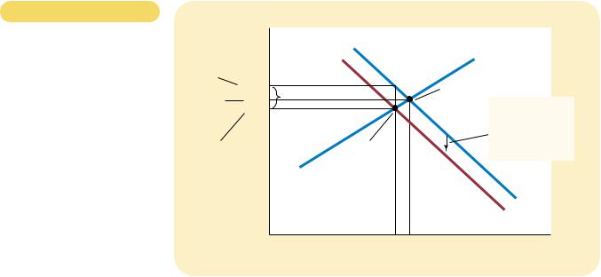
Figur e 6-6
A TAX ON BUYERS. When a tax of $0.50 is levied on buyers, the demand curve shifts down by $0.50 from D1 to D2. The equilibrium quantity falls from 100 to 90 cones. The price that sellers receive falls from $3.00 to $2.80. The price that buyers pay (including the tax) rises from $3.00 to $3.30. Even though the tax is levied on buyers, buyers and sellers share the burden of the tax.
Price of
Ice-Cream
Price Cone buyers
pay
|
$3.30 |
Tax ($0.50) |
|
Price |
3.00 |
||
|
|||
without |
2.80 |
|
|
|
|
||
tax |
|
|
|
Price |
|
Equilibrium |
|
sellers |
|
||
|
with tax |
||
receive |
|
||
|
|
Supply, S1
Equilibrium without tax
A tax on buyers shifts the demand curve downward by the size of
the tax ($0.50).
D1
D2
0 |
90 100 |
Quantity of |
|
|
Ice-Cream Cones |
130 |
PART TWO SUPPLY AND DEMAND I: HOW MARKETS WORK |
We can, in this case, be precise about how much the curve shifts. Because of the $0.50 tax levied on buyers, the effective price to buyers is now $0.50 higher than the market price. For example, if the market price of a cone happened to be $2.00, the effective price to buyers would be $2.50. Because buyers look at their total cost including the tax, they demand a quantity of ice cream as if the market price were $0.50 higher than it actually is. In other words, to induce buyers to demand any given quantity, the market price must now be $0.50 lower to make up for the effect of the tax. Thus, the tax shifts the demand curve downward from D1 to D2 by exactly the size of the tax ($0.50).
To see the effect of the tax, we compare the old equilibrium and the new equilibrium. You can see in the figure that the equilibrium price of ice cream falls from $3.00 to $2.80 and the equilibrium quantity falls from 100 to 90 cones. Because sellers sell less and buyers buy less in the new equilibrium, the tax on ice cream reduces the size of the ice-cream market.
Now let’s return to the question of tax incidence: Who pays the tax? Although buyers send the entire tax to the government, buyers and sellers share the burden. Because the market price falls from $3.00 to $2.80 when the tax is introduced, sellers receive $0.20 less for each ice-cream cone than they did without the tax. Thus, the tax makes sellers worse off. Buyers pay sellers a lower price ($2.80), but the effective price including the tax rises from $3.00 before the tax to $3.30 with the tax ($2.80 + $0.50 = $3.30). Thus, the tax also makes buyers worse off.
To sum up, the analysis yields two general lessons:
Taxes discourage market activity. When a good is taxed, the quantity of the good sold is smaller in the new equilibrium.
Buyers and sellers share the burden of taxes. In the new equilibrium, buyers pay more for the good, and sellers receive less.
HOW TAXES ON SELLERS AFFECT MARKET OUTCOMES
Now consider a tax levied on sellers of a good. Suppose the local government passes a law requiring sellers of ice-cream cones to send $0.50 to the government for each cone they sell. What are the effects of this law?
In this case, the initial impact of the tax is on the supply of ice cream. Because the tax is not levied on buyers, the quantity of ice cream demanded at any given price is the same, so the demand curve does not change. By contrast, the tax on sellers raises the cost of selling ice cream, and leads sellers to supply a smaller quantity at every price. The supply curve shifts to the left (or, equivalently, upward).
Once again, we can be precise about the magnitude of the shift. For any market price of ice cream, the effective price to sellers—the amount they get to keep after paying the tax—is $0.50 lower. For example, if the market price of a cone happened to be $2.00, the effective price received by sellers would be $1.50. Whatever the market price, sellers will supply a quantity of ice cream as if the price were $0.50 lower than it is. Put differently, to induce sellers to supply any given quantity, the market price must now be $0.50 higher to compensate for the effect of the tax. Thus, as shown in Figure 6-7, the supply curve shifts upward from S1 to S2 by exactly the size of the tax ($0.50).
When the market moves from the old to the new equilibrium, the equilibrium price of ice cream rises from $3.00 to $3.30, and the equilibrium quantity falls from
CHAPTER 6 SUPPLY, DEMAND, AND GOVERNMENT POLICIES |
131 |
|
Price of |
|
|
Ice-Cream |
|
||
Price |
Cone |
Equilibrium |
|
buyers |
|||
|
with tax |
||
pay |
|
||
$3.30 |
|
||
|
Tax ($0.50) |
||
Price |
3.00 |
||
|
|||
without |
2.80 |
|
|
|
|
||
tax |
|
|
|
Price |
|
|
|
sellers |
|
|
|
receive |
|
|
|
|
|
|
|
A tax on sellers S2 shifts the supply
curve upward
S1 by the amount of the tax ($0.50).
Equilibrium without tax
Demand, D1
0 |
90 100 |
Quantity of |
|
|
Ice-Cream Cones |
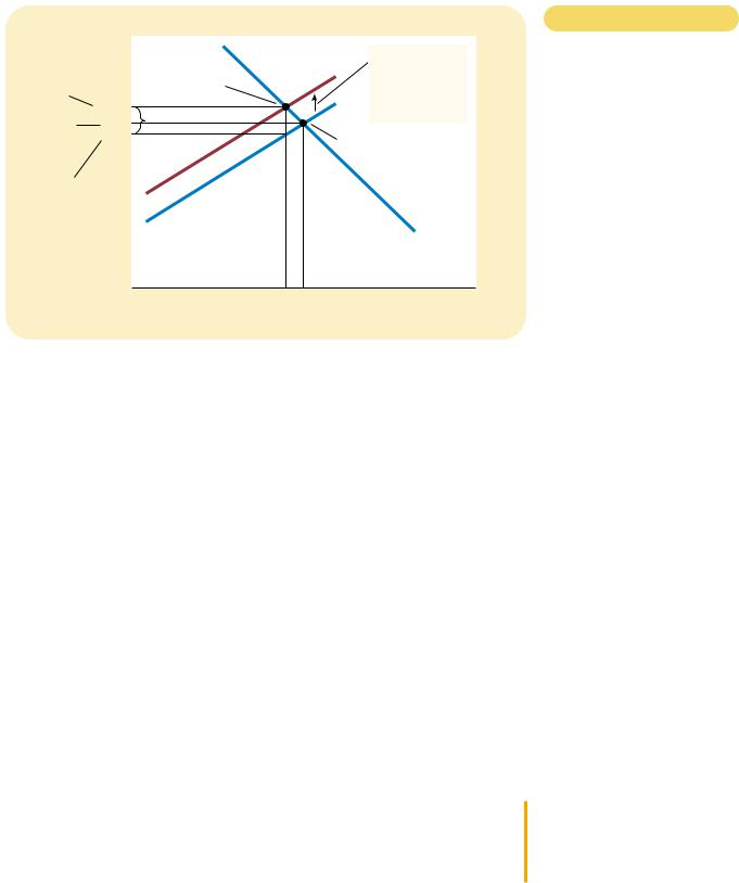
Figur e 6-7
A TAX ON SELLERS. When a tax of $0.50 is levied on sellers, the supply curve shifts up by $0.50 from S1 to S2. The equilibrium quantity falls from 100 to 90 cones. The price that buyers pay rises from $3.00 to $3.30. The price that sellers receive (after paying the tax) falls from $3.00 to $2.80. Even though the tax is levied on sellers, buyers and sellers share the burden of
the tax.
100 to 90 cones. Once again, the tax reduces the size of the ice-cream market. And once again, buyers and sellers share the burden of the tax. Because the market price rises, buyers pay $0.30 more for each cone than they did before the tax was enacted. Sellers receive a higher price than they did without the tax, but the effective price (after paying the tax) falls from $3.00 to $2.80.
Comparing Figures 6-6 and 6-7 leads to a surprising conclusion: Taxes on buyers and taxes on sellers are equivalent. In both cases, the tax places a wedge between the price that buyers pay and the price that sellers receive. The wedge between the buyers’ price and the sellers’ price is the same, regardless of whether the tax is levied on buyers or sellers. In either case, the wedge shifts the relative position of the supply and demand curves. In the new equilibrium, buyers and sellers share the burden of the tax. The only difference between taxes on buyers and taxes on sellers is who sends the money to the government.
The equivalence of these two taxes is perhaps easier to understand if we imagine that the government collects the $0.50 ice-cream tax in a bowl on the counter of each ice-cream store. When the government levies the tax on buyers, the buyer is required to place $0.50 in the bowl every time a cone is bought. When the government levies the tax on sellers, the seller is required to place $0.50 in the bowl after the sale of each cone. Whether the $0.50 goes directly from the buyer’s pocket into the bowl, or indirectly from the buyer’s pocket into the seller’s hand and then into the bowl, does not matter. Once the market reaches its new equilibrium, buyers and sellers share the burden, regardless of how the tax is levied.
CASE STUDY CAN CONGRESS DISTRIBUTE THE
BURDEN OF A PAYROLL TAX?
If you have ever received a paycheck, you probably noticed that taxes were deducted from the amount you earned. One of these taxes is called FICA, an
132 |
PART TWO SUPPLY AND DEMAND I: HOW MARKETS WORK |
acronym for the Federal Insurance Contribution Act. The federal government uses the revenue from the FICA tax to pay for Social Security and Medicare, the income support and health care programs for the elderly. FICA is an example of a payroll tax, which is a tax on the wages that firms pay their workers. In 1999, the total FICA tax for the typical worker was 15.3 percent of earnings.
Who do you think bears the burden of this payroll tax—firms or workers? When Congress passed this legislation, it attempted to mandate a division of the tax burden. According to the law, half of the tax is paid by firms, and half is paid by workers. That is, half of the tax is paid out of firm revenue, and half is deducted from workers’ paychecks. The amount that shows up as a deduction on your pay stub is the worker contribution.
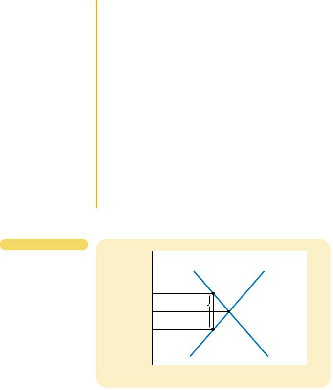
Our analysis of tax incidence, however, shows that lawmakers cannot so easily distribute the burden of a tax. To illustrate, we can analyze a payroll tax as merely a tax on a good, where the good is labor and the price is the wage. The key feature of the payroll tax is that it places a wedge between the wage that firms pay and the wage that workers receive. Figure 6-8 shows the outcome. When a payroll tax is enacted, the wage received by workers falls, and the wage paid by firms rises. In the end, workers and firms share the burden of the tax, much as the legislation requires. Yet this division of the tax burden between workers and firms has nothing to do with the legislated division: The division of the burden in Figure 6-8 is not necessarily fifty-fifty, and the same outcome would prevail if the law levied the entire tax on workers or if it levied the entire tax on firms.
This example shows that the most basic lesson of tax incidence is often overlooked in public debate. Lawmakers can decide whether a tax comes from the buyer’s pocket or from the seller’s, but they cannot legislate the true burden of a tax. Rather, tax incidence depends on the forces of supply and demand.
Figur e 6-8
A PAYROLL TAX. A payroll tax places a wedge between the wage that workers receive and the wage that firms pay. Comparing wages with and without the tax, you can see that workers and firms share the tax burden. This division of the tax burden between workers and firms does not depend on whether the government levies the tax on workers, levies the tax on firms, or divides the tax equally between the two groups.
Wage |
|
|
Labor supply |
Wage firms pay |
|
|
Tax wedge |
Wage without tax |
|
Wage workers |
|
receive |
|
|
Labor demand |
0 |
Quantity |
|
of Labor |
CHAPTER 6 SUPPLY, DEMAND, AND GOVERNMENT POLICIES |
133 |
ELASTICITY AND TAX INCIDENCE
When a good is taxed, buyers and sellers of the good share the burden of the tax. But how exactly is the tax burden divided? Only rarely will it be shared equally. To see how the burden is divided, consider the impact of taxation in the two markets in Figure 6-9. In both cases, the figure shows the initial demand curve, the initial supply curve, and a tax that drives a wedge between the amount paid by buyers and the amount received by sellers. (Not drawn in either panel of the figure is the new supply or demand curve. Which curve shifts depends on whether the tax is levied on buyers or sellers. As we have seen, this is irrelevant for the incidence of
Price
Price buyers pay
Price without tax
Price sellers receive
0
Price
Price buyers pay
Price without tax
Price sellers receive
(a)Elastic Supply, Inelastic Demand
1.When supply is more elastic than demand . . .
Supply
Tax
2. . . . the incidence of the tax falls more heavily on consumers . . .
3. . . . than
Demand
on producers.
Quantity
(b) Inelastic Supply, Elastic Demand
1. When demand is more elastic than supply . . .
Supply
3. . . . than on consumers.
Tax
2. . . . the |
Demand |
|
incidence of |
||
|
||
the tax falls |
|
|
more heavily |
|
|
on producers . . . |
|
|
|
|
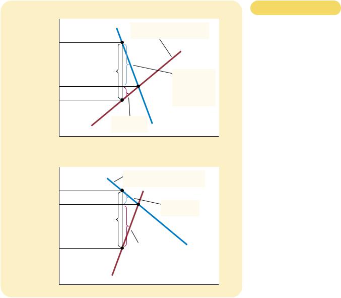
Figur e 6-9
HOW THE BURDEN OF A TAX IS
DIVIDED. In panel (a), the supply curve is elastic, and the demand curve is inelastic. In this case, the price received by sellers falls only slightly, while the price paid by buyers rises substantially. Thus, buyers bear most of the burden of the tax. In panel (b), the supply curve is inelastic, and the demand curve is elastic. In this case, the price received by sellers falls substantially, while the price paid by buyers rises only slightly. Thus, sellers bear most of the burden of the tax.
0 |
Quantity |

134 |
PART TWO SUPPLY AND DEMAND I: HOW MARKETS WORK |
the tax.) The difference in the two panels is the relative elasticity of supply and demand.
Panel (a) of Figure 6-9 shows a tax in a market with very elastic supply and relatively inelastic demand. That is, sellers are very responsive to the price of the good, whereas buyers are not very responsive. When a tax is imposed on a market with these elasticities, the price received by sellers does not fall much, so sellers bear only a small burden. By contrast, the price paid by buyers rises substantially, indicating that buyers bear most of the burden of the tax.
Panel (b) of Figure 6-9 shows a tax in a market with relatively inelastic supply and very elastic demand. In this case, sellers are not very responsive to the price, while buyers are very responsive. The figure shows that when a tax is imposed, the price paid by buyers does not rise much, while the price received by sellers falls substantially. Thus, sellers bear most of the burden of the tax.
The two panels of Figure 6-9 show a general lesson about how the burden of a tax is divided: A tax burden falls more heavily on the side of the market that is less elastic. Why is this true? In essence, the elasticity measures the willingness of buyers or sellers to leave the market when conditions become unfavorable. A small elasticity of demand means that buyers do not have good alternatives to consuming this particular good. A small elasticity of supply means that sellers do not have good alternatives to producing this particular good. When the good is taxed, the side of the market with fewer good alternatives cannot easily leave the market and must, therefore, bear more of the burden of the tax.
We can apply this logic to the payroll tax, which was discussed in the previous case study. Most labor economists believe that the supply of labor is much less elastic than the demand. This means that workers, rather than firms, bear most of the burden of the payroll tax. In other words, the distribution of the tax burden is not at all close to the fifty-fifty split that lawmakers intended.
“IF THIS BOAT WERE ANY MORE EXPENSIVE, WE WOULD BE PLAYING GOLF.”
CASE STUDY WHO PAYS THE LUXURY TAX?
In 1990, Congress adopted a new luxury tax on items such as yachts, private airplanes, furs, jewelry, and expensive cars. The goal of the tax was to raise revenue from those who could most easily afford to pay. Because only the rich could afford to buy such extravagances, taxing luxuries seemed a logical way of taxing the rich.
Yet, when the forces of supply and demand took over, the outcome was quite different from what Congress intended. Consider, for example, the market for yachts. The demand for yachts is quite elastic. A millionaire can easily not buy a yacht; she can use the money to buy a bigger house, take a European vacation, or leave a larger bequest to her heirs. By contrast, the supply of yachts is relatively inelastic, at least in the short run. Yacht factories are not easily converted to alternative uses, and workers who build yachts are not eager to change careers in response to changing market conditions.
Our analysis makes a clear prediction in this case. With elastic demand and inelastic supply, the burden of a tax falls largely on the suppliers. That is, a tax on yachts places a burden largely on the firms and workers who build yachts because they end up getting a lower price for their product. The workers, however, are not wealthy. Thus, the burden of a luxury tax falls more on the middle class than on the rich.