

principles_of_economics_gregory_mankiw
.pdfCHAPTER 5 ELASTICITY AND ITS APPLICATION |
105 |
responds substantially to changes in the price. Supply is said to be inelastic if the quantity supplied responds only slightly to changes in the price.
The price elasticity of supply depends on the flexibility of sellers to change the amount of the good they produce. For example, beachfront land has an inelastic supply because it is almost impossible to produce more of it. By contrast, manufactured goods, such as books, cars, and televisions, have elastic supplies because the firms that produce them can run their factories longer in response to a higher price.
In most markets, a key determinant of the price elasticity of supply is the time period being considered. Supply is usually more elastic in the long run than in the short run. Over short periods of time, firms cannot easily change the size of their factories to make more or less of a good. Thus, in the short run, the quantity supplied is not very responsive to the price. By contrast, over longer periods, firms can build new factories or close old ones. In addition, new firms can enter a market, and old firms can shut down. Thus, in the long run, the quantity supplied can respond substantially to the price.
COMPUTING THE PRICE ELASTICITY OF SUPPLY
Now that we have some idea about what the price elasticity of supply is, let’s be more precise. Economists compute the price elasticity of supply as the percentage change in the quantity supplied divided by the percentage change in the price. That is,
Price elasticity of supply |
Percentage change in quantity supplied |
. |
|
Percentage change in price |
|||
|
|
For example, suppose that an increase in the price of milk from $2.85 to $3.15 a gallon raises the amount that dairy farmers produce from 9,000 to 11,000 gallons per month. Using the midpoint method, we calculate the percentage change in price as
Percentage change in price (3.15 2.85)/3.00 100 10 percent.
Similarly, we calculate the percentage change in quantity supplied as
Percentage change in quantity supplied (11,000 9,000)/10,000 10020 percent.
In this case, the price elasticity of supply is
20 percent
Price elasticity of supply 10 percent 2.0.
In this example, the elasticity of 2 reflects the fact that the quantity supplied moves proportionately twice as much as the price.
THE VARIETY OF SUPPLY CURVES
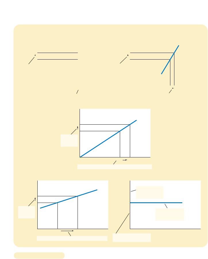
Because the price elasticity of supply measures the responsiveness of quantity supplied to the price, it is reflected in the appearance of the supply curve. Figure 5-6 shows five cases. In the extreme case of a zero elasticity, supply is perfectly inelastic,
|
|
(a) Perfectly Inelastic Supply: Elasticity Equals 0 |
|
|
|
|
(b) Inelastic Supply: Elasticity Is Less Than 1 |
|||||||
Price |
|
|
|
|
|
Price |
|
|
|
|
|
|
||
|
|
Supply |
|
|
|
|
Supply |
|
|
|||||
|
|
|
|
|
|
|
|
|
|
|
|
|
||
|
|
|
|
|
|
|
|
|
|
|
|
|
||
|
|
|
|
|
|
|
|
|
|
|
|
|
|
|
$5 |
|
|
|
|
$5 |
|
|
|
|
|
|
|||
|
|
|
|
|
|
|
|
|
|
|
|
|
|
|
|
|
|
|
|
|
|
|
|
|
|
|
|
|
|
4 |
|
|
|
|
4 |
|
|
|
|
|
|
|||
|
|
|
|
|
|
|
|
|
|
|
|
|
|
|
1. An |
|
|
|
|
|
|
1. A 22% |
|
|
|
|
|
|
|
increase |
|
|
|
|
|
|
increase |
|
|
|
|
|
|
|
in price . . . |
|
|
|
|
|
|
in price . . . |
|
|
|
|
|
|
|
|
|
|
|
|
|
|
|
|
|
|
|
|
|
|
0 |
100 |
Quantity |
0 |
100 |
|
110 |
Quantity |
|||||||
|
||||||||||||||
|
|
|
|
|
|
|
|
|
||||||
|
|
|
2. . . . leaves the quantity supplied unchanged. |
|
|
|
|
2. . . . leads to a 10% increase in quantity supplied. |
||||||
|
|
|
|
|
|
|
|
|
|
|
|
|
|
|
(c) Unit Elastic Supply: Elasticity Equals 1
Price |
|
|
|
|
|
|
Supply |
$5 |
|
|
|
4 |
|
|
|
1. A 22% |
|
|
|
increase |
|
|
|
in price . . . |
|
|
|
0 |
100 |
125 |
Quantity |
2. |
. . . leads to a 22% increase in quantity supplied. |
||
(d) Elastic Supply: Elasticity Is Greater Than 1 |
(e) Perfectly Elastic Supply: Elasticity Equals Infinity |
Price |
|
|
|
Price |
|
|
|
|
Supply |
1. At any price |
|
$5 |
|
|
|
above $4, quantity |
|
|
|
|
supplied is infinite. |
|
|
4 |
|
|
|
$4 |
Supply |
1. A 22% |
|
|
|
2. At exactly $4, |
|
increase |
|
|
|
|
|
|
|
|
producers will |
|
|
in price . . . |
|
|
|
|
|
|
|
|
supply any quantity. |
|
|
|
|
|
|
|
|
0 |
100 |
200 |
Quantity |
0 |
Quantity |
|
2. . . . leads to a 67% increase in quantity supplied. |
3. At a price below $4, |
|
||
|
quantity supplied is zero. |
|
|||
|
|
|
|
|
|
Figur e 5-6 |
|
THE PRICE ELASTICITY OF SUPPLY. The price elasticity of supply determines whether the |
|
supply curve is steep or flat. Note that all percentage changes are calculated using the |
|
|
|
|
|
|
midpoint method. |
|
|
|
CHAPTER 5 ELASTICITY AND ITS APPLICATION |
107 |
Price |
|
|
|
|
|
$15 |
|
|
|
|
|
|
|
|
Elasticity is small |
|
|
|
|
|
(less than 1). |
|
|
12 |
|
|
|
|
|
|
Elasticity is large |
|
|
|
|
|
(greater than 1). |
|
|
|
|
4 |
|
|
|
|
|
3 |
|
|
|
|
|
0 |
100 |
200 |
500 |
525 |
Quantity |
and the supply curve is vertical. In this case, the quantity supplied is the same regardless of the price. As the elasticity rises, the supply curve gets flatter, which shows that the quantity supplied responds more to changes in the price. At the opposite extreme, supply is perfectly elastic. This occurs as the price elasticity of supply approaches infinity and the supply curve becomes horizontal, meaning that very small changes in the price lead to very large changes in the quantity supplied.
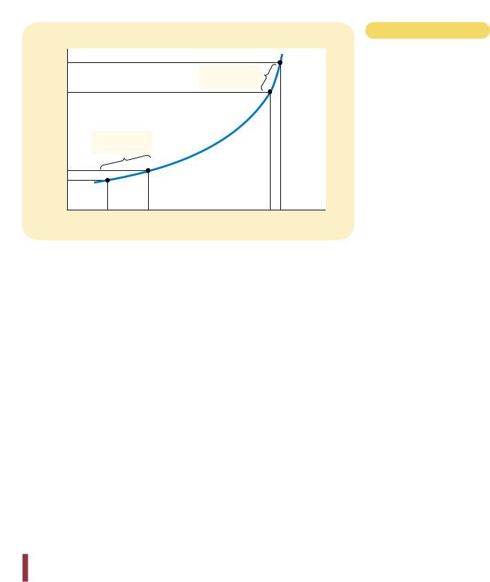
In some markets, the elasticity of supply is not constant but varies over the supply curve. Figure 5-7 shows a typical case for an industry in which firms have factories with a limited capacity for production. For low levels of quantity supplied, the elasticity of supply is high, indicating that firms respond substantially to changes in the price. In this region, firms have capacity for production that is not being used, such as plants and equipment sitting idle for all or part of the day. Small increases in price make it profitable for firms to begin using this idle capacity. As the quantity supplied rises, firms begin to reach capacity. Once capacity is fully used, increasing production further requires the construction of new plants. To induce firms to incur this extra expense, the price must rise substantially, so supply becomes less elastic.
Figure 5-7 presents a numerical example of this phenomenon. When the price rises from $3 to $4 (a 29 percent increase, according to the midpoint method), the quantity supplied rises from 100 to 200 (a 67 percent increase). Because quantity supplied moves proportionately more than the price, the supply curve has elasticity greater than 1. By contrast, when the price rises from $12 to $15 (a 22 percent increase), the quantity supplied rises from 500 to 525 (a 5 percent increase). In this case, quantity supplied moves proportionately less than the price, so the elasticity is less than 1.
QUICK QUIZ: Define the price elasticity of supply. Explain why the the price elasticity of supply might be different in the long run than in the short run.
Figur e 5-7
HOW THE PRICE ELASTICITY OF
SUPPLY CAN VARY. Because firms often have a maximum capacity for production, the elasticity of supply may be very high at low levels of quantity supplied and very low at high levels of quantity supplied. Here, an increase in price from $3 to $4 increases the quantity supplied from 100 to 200. Because the increase in quantity supplied of 67 percent is larger than the increase in price of 29 percent, the supply curve is elastic in this range. By contrast, when the price rises from $12 to $15, the quantity supplied rises only from 500 to 525. Because the increase in quantity supplied of 5 percent is smaller than the increase in price of 22 percent, the supply curve is inelastic in this range.

108 |
PART TWO SUPPLY AND DEMAND I: HOW MARKETS WORK |
THREE APPLICATIONS OF SUPPLY,
DEMAND, AND ELASTICITY
Can good news for farming be bad news for farmers? Why did the Organization of Petroleum Exporting Countries (OPEC) fail to keep the price of oil high? Does drug interdiction increase or decrease drug-related crime? At first, these questions might seem to have little in common. Yet all three questions are about markets, and all markets are subject to the forces of supply and demand. Here we apply the versatile tools of supply, demand, and elasticity to answer these seemingly complex questions.
CAN GOOD NEWS FOR FARMING BE
BAD NEWS FOR FARMERS?
Let’s now return to the question posed at the beginning of this chapter: What happens to wheat farmers and the market for wheat when university agronomists discover a new wheat hybrid that is more productive than existing varieties? Recall from Chapter 4 that we answer such questions in three steps. First, we examine whether the supply curve or demand curve shifts. Second, we consider which direction the curve shifts. Third, we use the supply-and-demand diagram to see how the market equilibrium changes.
In this case, the discovery of the new hybrid affects the supply curve. Because the hybrid increases the amount of wheat that can be produced on each acre of land, farmers are now willing to supply more wheat at any given price. In other words, the supply curve shifts to the right. The demand curve remains the same because consumers’ desire to buy wheat products at any given price is not affected by the introduction of a new hybrid. Figure 5-8 shows an example of such a change. When the supply curve shifts from S1 to S2, the quantity of wheat sold increases from 100 to 110, and the price of wheat falls from $3 to $2.
But does this discovery make farmers better off? As a first cut to answering this question, consider what happens to the total revenue received by farmers. Farmers’ total revenue is P Q, the price of the wheat times the quantity sold. The discovery affects farmers in two conflicting ways. The hybrid allows farmers to produce more wheat (Q rises), but now each bushel of wheat sells for less (P falls).
Whether total revenue rises or falls depends on the elasticity of demand. In practice, the demand for basic foodstuffs such as wheat is usually inelastic, for these items are relatively inexpensive and have few good substitutes. When the demand curve is inelastic, as it is in Figure 5-8, a decrease in price causes total revenue to fall. You can see this in the figure: The price of wheat falls substantially, whereas the quantity of wheat sold rises only slightly. Total revenue falls from $300 to $220. Thus, the discovery of the new hybrid lowers the total revenue that farmers receive for the sale of their crops.
If farmers are made worse off by the discovery of this new hybrid, why do they adopt it? The answer to this question goes to the heart of how competitive markets work. Because each farmer is a small part of the market for wheat, he or she takes the price of wheat as given. For any given price of wheat, it is better to

Price of
Wheat
2. . . . leads $3 to a large
fall in
price . . . 2
0
CHAPTER 5 ELASTICITY AND ITS APPLICATION |
109 |
1. When demand is inelastic, an increase in supply . . .
S1
S2
Demand
Figur e 5-8
AN INCREASE IN SUPPLY IN THE MARKET FOR WHEAT. When an
advance in farm technology increases the supply of wheat from S1 to S2, the price of wheat falls. Because the demand for wheat is inelastic, the increase in the quantity sold from 100 to 110 is proportionately smaller than the decrease in the price from $3 to $2. As a result, farmers’ total revenue falls from $300
($3 100) to $220 ($2 110).
100  110 Quantity of Wheat
3. . . . and a proportionately smaller increase in quantity sold. As a result, revenue falls from $300 to $220.
use the new hybrid in order to produce and sell more wheat. Yet when all farmers do this, the supply of wheat rises, the price falls, and farmers are worse off.
Although this example may at first seem only hypothetical, in fact it helps to explain a major change in the U.S. economy over the past century. Two hundred years ago, most Americans lived on farms. Knowledge about farm methods was sufficiently primitive that most of us had to be farmers to produce enough food. Yet, over time, advances in farm technology increased the amount of food that each farmer could produce. This increase in food supply, together with inelastic food demand, caused farm revenues to fall, which in turn encouraged people to leave farming.
A few numbers show the magnitude of this historic change. As recently as 1950, there were 10 million people working on farms in the United States, representing 17 percent of the labor force. In 1998, fewer than 3 million people worked on farms, or 2 percent of the labor force. This change coincided with tremendous advances in farm productivity: Despite the 70 percent drop in the number of farmers, U.S. farms produced more than twice the output of crops and livestock in 1998 as they did in 1950.
This analysis of the market for farm products also helps to explain a seeming paradox of public policy: Certain farm programs try to help farmers by inducing them not to plant crops on all of their land. Why do these programs do this? Their purpose is to reduce the supply of farm products and thereby raise prices. With inelastic demand for their products, farmers as a group receive greater total revenue if they supply a smaller crop to the market. No single farmer would choose to leave his land fallow on his own because each takes the market price as given. But if all farmers do so together, each of them can be better off.

110 |
PART TWO SUPPLY AND DEMAND I: HOW MARKETS WORK |
When analyzing the effects of farm technology or farm policy, it is important to keep in mind that what is good for farmers is not necessarily good for society as a whole. Improvement in farm technology can be bad for farmers who become increasingly unnecessary, but it is surely good for consumers who pay less for food. Similarly, a policy aimed at reducing the supply of farm products may raise the incomes of farmers, but it does so at the expense of consumers.
WHY DID OPEC FAIL TO KEEP THE PRICE OF OIL HIGH?
Many of the most disruptive events for the world’s economies over the past several decades have originated in the world market for oil. In the 1970s members of the Organization of Petroleum Exporting Countries (OPEC) decided to raise the world price of oil in order to increase their incomes. These countries accomplished this goal by jointly reducing the amount of oil they supplied. From 1973 to 1974, the price of oil (adjusted for overall inflation) rose more than 50 percent. Then, a few years later, OPEC did the same thing again. The price of oil rose 14 percent in 1979, followed by 34 percent in 1980, and another 34 percent in 1981.
Yet OPEC found it difficult to maintain a high price. From 1982 to 1985, the price of oil steadily declined at about 10 percent per year. Dissatisfaction and disarray soon prevailed among the OPEC countries. In 1986 cooperation among OPEC members completely broke down, and the price of oil plunged 45 percent. In 1990 the price of oil (adjusted for overall inflation) was back to where it began in 1970, and it has stayed at that low level throughout most of the 1990s.
This episode shows how supply and demand can behave differently in the short run and in the long run. In the short run, both the supply and demand for oil are relatively inelastic. Supply is inelastic because the quantity of known oil reserves and the capacity for oil extraction cannot be changed quickly. Demand is inelastic because buying habits do not respond immediately to changes in price. Many drivers with old gas-guzzling cars, for instance, will just pay the higher

|
|
|
|
|
|
|
|
|
|
CHAPTER 5 |
ELASTICITY AND ITS APPLICATION |
111 |
|||||||||
|
|
|
|
(a) The Oil Market in the Short Run |
|
|
|
|
|
(b) The Oil Market in the Long Run |
|
||||||||||
Price of Oil |
|
|
|
|
|
|
Price of Oil |
|
|
|
|
|
|
|
|||||||
|
|
|
|
|
|
|
|
|
|
|
|
|
|||||||||
|
|
|
|
|
1. In the short run, when supply |
|
|
|
|
|
|
|
|
|
|
|
|
|
|
||
|
|
|
|
|
|
|
|
|
|
|
|
|
1. In the long run, |
|
|
|
|||||
|
|
|
|
|
and demand are inelastic, |
|
|
|
|
|
|
|
|
when supply and |
|
|
|
||||
|
|
|
|
|
a shift in supply . . . |
|
|
|
|
|
|
|
|
demand are elastic, |
|
|
|
||||
|
|
|
|
|
|
S2 |
|
|
|
|
|
|
|
a shift in supply . . . |
|
|
|
||||
|
|
|
|
|
|
|
S1 |
|
|
|
|
|
|
|
|
|
S2 |
|
|
||
|
|
|
|
|
|
|
|
|
|
|
|
|
|
|
|
|
|
|
|
||
|
|
|
|
|
|
|
|
|
|
|
|
|
|
|
|
|
|
|
S1 |
|
|
|
P2 |
|
|
|
|
|
|
|
|
|
|
|
|
|
|
|
|
|
|
||
|
|
|
|
|
|
|
2. . . . leads |
|
|
|
|
|
|
|
|
|
|
|
|||
2. . . . leads |
|
|
|
|
|
|
P2 |
|
|
|
|
|
|
|
|||||||
|
|
|
|
|
|
|
|
|
|
|
|
|
|
|
|
||||||
|
|
|
|
|
|
|
|
|
to a small |
|
|
|
|
|
|
|
|||||
to a large |
|
|
|
|
|
|
|
|
|
|
|
|
|
|
|
|
|||||
|
|
|
|
|
|
|
|
|
increase |
|
|
|
|
|
|
|
|
|
|
|
|
|
|
|
|
|
|
|
|
|
|
|
|
|
|
|
|
|
|
|
|
||
increase |
|
|
|
|
|
|
|
|
|
P1 |
|
|
|
|
|
|
|
||||
P1 |
|
|
|
|
|
|
in price. |
|
|
|
|
|
|
|
|||||||
in price. |
|
|
|
|
|
|
|
|
|
|
|
|
|
|
|
|
|
||||
|
|
|
|
|
|
|
|
|
|
|
|
|
|
|
|
|
Demand |
|
|
||
|
|
|
|
|
|
|
|
|
|
|
|
|
|
|
|
|
|
|
|
||
|
|
|
|
|
|
|
Demand |
|
|
|
|
|
|
|
|
|
|
|
|
|
|
|
|
|
|
|
|
|
|
|
|
|
|
|
|
|
|
|
|
|
|
|
|
|
0 |
|
|
|
Quantity of Oil |
|
0 |
|
|
|
|
|
Quantity of Oil |
|
|||||||
A REDUCTION IN SUPPLY IN THE WORLD MARKET FOR OIL. When the supply of oil falls,
the response depends on the time horizon. In the short run, supply and demand are relatively inelastic, as in panel (a). Thus, when the supply curve shifts from S1 to S2, the price rises substantially. By contrast, in the long run, supply and demand are relatively elastic, as in panel (b). In this case, the same size shift in the supply curve (S1 to S2) causes a smaller increase in the price.
Figur e 5-9
price. Thus, as panel (a) of Figure 5-9 shows, the short-run supply and demand curves are steep. When the supply of oil shifts from S1 to S2, the price increase from P1 to P2 is large.
The situation is very different in the long run. Over long periods of time, producers of oil outside of OPEC respond to high prices by increasing oil exploration and by building new extraction capacity. Consumers respond with greater conservation, for instance by replacing old inefficient cars with newer efficient ones. Thus, as panel (b) of Figure 5-9 shows, the long-run supply and demand curves are more elastic. In the long run, the shift in the supply curve from S1 to S2 causes a much smaller increase in the price.
This analysis shows why OPEC succeeded in maintaining a high price of oil only in the short run. When OPEC countries agreed to reduce their production of oil, they shifted the supply curve to the left. Even though each OPEC member sold less oil, the price rose by so much in the short run that OPEC incomes rose. By contrast, in the long run when supply and demand are more elastic, the same reduction in supply, measured by the horizontal shift in the supply curve, caused a smaller increase in the price. Thus, OPEC’s coordinated reduction in supply proved less profitable in the long run.
OPEC still exists today, and it has from time to time succeeded at reducing supply and raising prices. But the price of oil (adjusted for overall inflation) has
112 |
PART TWO SUPPLY AND DEMAND I: HOW MARKETS WORK |
never returned to the peak reached in 1981. The cartel now seems to understand that raising prices is easier in the short run than in the long run.
DOES DRUG INTERDICTION INCREASE
OR DECREASE DRUG-RELATED CRIME?
A persistent problem facing our society is the use of illegal drugs, such as heroin, cocaine, and crack. Drug use has several adverse effects. One is that drug dependency can ruin the lives of drug users and their families. Another is that drug addicts often turn to robbery and other violent crimes to obtain the money needed to support their habit. To discourage the use of illegal drugs, the U.S. government devotes billions of dollars each year to reduce the flow of drugs into the country. Let’s use the tools of supply and demand to examine this policy of drug interdiction.
Suppose the government increases the number of federal agents devoted to the war on drugs. What happens in the market for illegal drugs? As is usual, we answer this question in three steps. First, we consider whether the supply curve or demand curve shifts. Second, we consider the direction of the shift. Third, we see how the shift affects the equilibrium price and quantity.
Although the purpose of drug interdiction is to reduce drug use, its direct impact is on the sellers of drugs rather than the buyers. When the government stops some drugs from entering the country and arrests more smugglers, it raises the cost of selling drugs and, therefore, reduces the quantity of drugs supplied at any given price. The demand for drugs—the amount buyers want at any given price— is not changed. As panel (a) of Figure 5-10 shows, interdiction shifts the supply curve to the left from S1 to S2 and leaves the demand curve the same. The equilibrium price of drugs rises from P1 to P2, and the equilibrium quantity falls from Q1 to Q2. The fall in the equilibrium quantity shows that drug interdiction does reduce drug use.
But what about the amount of drug-related crime? To answer this question, consider the total amount that drug users pay for the drugs they buy. Because few drug addicts are likely to break their destructive habits in response to a higher price, it is likely that the demand for drugs is inelastic, as it is drawn in the figure. If demand is inelastic, then an increase in price raises total revenue in the drug market. That is, because drug interdiction raises the price of drugs proportionately more than it reduces drug use, it raises the total amount of money that drug users pay for drugs. Addicts who already had to steal to support their habits would have an even greater need for quick cash. Thus, drug interdiction could increase drug-related crime.
Because of this adverse effect of drug interdiction, some analysts argue for alternative approaches to the drug problem. Rather than trying to reduce the supply of drugs, policymakers might try to reduce the demand by pursuing a policy of drug education. Successful drug education has the effects shown in panel (b) of Figure 5-10. The demand curve shifts to the left from D1 to D2. As a result, the equilibrium quantity falls from Q1 to Q2, and the equilibrium price falls from P1 to P2. Total revenue, which is price times quantity, also falls. Thus, in contrast to drug interdiction, drug education can reduce both drug use and drug-related crime.
Advocates of drug interdiction might argue that the effects of this policy are different in the long run than in the short run, because the elasticity of demand may depend on the time horizon. The demand for drugs is probably inelastic over

CHAPTER 5 |
ELASTICITY AND ITS APPLICATION |
113 |
(a) Drug Interdiction |
(b) Drug Education |
|
Price of |
|
|
|
Price of |
|
|
|
Drugs |
1. Drug interdiction reduces |
Drugs |
1. Drug education reduces |
||||
|
|
||||||
|
|
the demand for drugs . . . |
|||||
|
the supply of drugs . . . |
|
|||||
|
|
|
|
|
|||
|
|
S2 |
|
|
|
|
Supply |
P2 |
|
|
S1 |
|
|
|
|
|
|
|
P1 |
|
|
|
|
P1 |
|
|
|
P2 |
|
|
|
2. . . . which |
|
|
|
2. . . . which |
|
|
|
raises the |
|
|
|
reduces the |
|
|
|
price . . . |
|
|
Demand |
price . . . |
|
|
D1 |
|
|
|
|
|
D2 |
||
|
|
|
|
|
|
|
|
0 |
Q2 |
Q1 |
Quantity of Drugs |
0 |
Q2 |
Q1 |
Quantity of Drugs |
 3. . . . and reduces the quantity sold.
POLICIES TO REDUCE THE USE OF ILLEGAL DRUGS. Drug interdiction reduces the supply of drugs from S1 to S2, as in panel (a). If the demand for drugs is inelastic, then the total amount paid by drug users rises, even as the amount of drug use falls. By contrast, drug education reduces the demand for drugs from D1 to D2, as in panel (b). Because both price and quantity fall, the amount paid by drug users falls.
short periods of time because higher prices do not substantially affect drug use by established addicts. But demand may be more elastic over longer periods of time because higher prices would discourage experimentation with drugs among the young and, over time, lead to fewer drug addicts. In this case, drug interdiction would increase drug-related crime in the short run while decreasing it in the long run.
QUICK QUIZ: How might a drought that destroys half of all farm crops be good for farmers? If such a drought is good for farmers, why don’t farmers destroy their own crops in the absence of a drought?
 3. . . . and reduces the quantity sold.
Figur e 5-10
CONCLUSION
According to an old quip, even a parrot can become an economist simply by learning to say “supply and demand.” These last two chapters should have convinced you that there is much truth in this statement. The tools of supply and demand allow you to analyze many of the most important events and policies that shape

114 |
PART TWO SUPPLY AND DEMAND I: HOW MARKETS WORK |
the economy. You are now well on your way to becoming an economist (or, at least, a well-educated parrot).
The price elasticity of demand quantity demanded responds to Demand tends to be more elastic rather than a necessity, if close
if the market is narrowly defined, substantial time to react to a price
The price elasticity of demand is percentage change in quantity the percentage change in price. than 1, so that quantity demanded proportionately less than the inelastic. If the elasticity is greater quantity demanded moves
the price, demand is said to be
Total revenue, the total amount the price of the good times the inelastic demand curves, total rises. For elastic demand curves, price rises.
The income elasticity of demand the quantity demanded responds
Summar y
The cross-price elasticity of demand the quantity demanded of one price of another good.
of supply measures how much the responds to changes in the price. This on the time horizon under
most markets, supply is more elastic in the short run.
of supply is calculated as the
in quantity supplied divided by the in price. If the elasticity is less than 1,
supplied moves proportionately less is said to be inelastic. If the
than 1, so that quantity supplied more than the price, supply is
and demand can be applied in many markets. This chapter uses them to
for wheat, the market for oil, and the drugs.
Key Concepts
elasticity, p. 94 |
-price elasticity of demand, p. 104 |
price elasticity of demand, p. 94 |
elasticity of supply, p. 104 |
Questions for Review
1.Define the price elasticity of demand and the income elasticity of demand.
2.List and explain some of the determinants of the price elasticity of demand.
3.If the elasticity is greater than 1, is demand elastic or inelastic? If the elasticity equals 0, is demand perfectly elastic or perfectly inelastic?
4.On a supply-and-demand diagram, show equilibrium price, equilibrium quantity, and the total revenue received by producers.
5.If demand is elastic, how will an increase in price change total revenue? Explain.
6.What do we call a good whose income elasticity is less than 0?
7.How is the price elasticity of supply calculated? Explain what this measures.
8.What is the price elasticity of supply of Picasso paintings?
9.Is the price elasticity of supply usually larger in the short run or in the long run? Why?
10.In the 1970s, OPEC caused a dramatic increase in the price of oil. What prevented it from maintaining this high price through the 1980s?