

principles_of_economics_gregory_mankiw
.pdfCHAPTER 8
(a) Inelastic Supply
Price |
Price |
Supply
When supply is relatively inelastic, the deadweight loss of a tax is small.
Size of tax
|
Demand |
|
0 |
Quantity |
0 |
|
(c) Inelastic Demand |
|
Price |
|
Price |
|
Supply |
|
Size of tax
When demand is relatively inelastic, the deadweight loss of a tax is small.
Demand
0 |
Quantity |
0 |
APPLICATION: THE COSTS OF TAXATION |
167 |
(b) Elastic Supply
When supply is relatively elastic, the deadweight loss of a tax is large.
Size |
Supply |
|
|
of |
|
tax |
|
Demand
Quantity
(d) Elastic Demand
Supply
Size |
|
of |
|
tax |
Demand |
When demand is relatively elastic, the deadweight loss of a tax is large.
Quantity
|
|
|
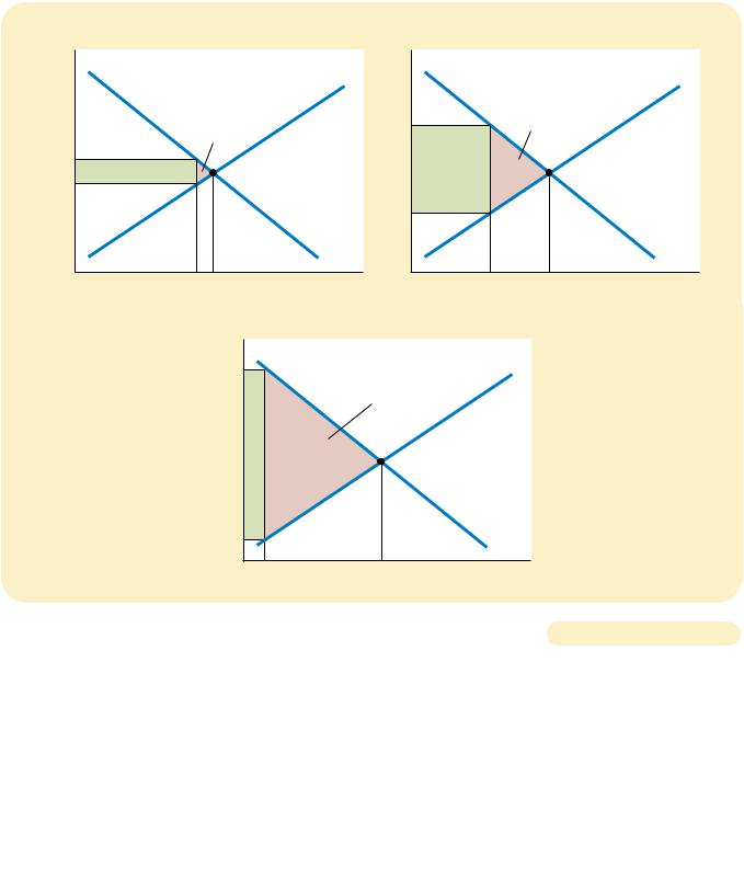
TAX DISTORTIONS AND ELASTICITIES. In panels (a) and (b), the demand curve and the |
Figur e 8-5 |
|
size of the tax are the same, but the price elasticity of supply is different. Notice that the |
|
|
|
|
|
more elastic the supply curve, the larger the deadweight loss of the tax. In panels (c) and |
|
|
(d), the supply curve and the size of the tax are the same, but the price elasticity of |
|
|
demand is different. Notice that the more elastic the demand curve, the larger the |
|
|
deadweight loss of the tax. |
|
|
|
|
|
|
|
|
Let’s consider first how the elasticity of supply affects the size of the deadweight loss. In the top two panels of Figure 8-5, the demand curve and the size of the tax are the same. The only difference in these figures is the elasticity of the supply curve. In panel (a), the supply curve is relatively inelastic: Quantity supplied responds only slightly to changes in the price. In panel (b), the supply curve is

168 |
PART THREE SUPPLY AND DEMAND II: MARKETS AND WELFARE |
relatively elastic: Quantity supplied responds substantially to changes in the price. Notice that the deadweight loss, the area of the triangle between the supply and demand curves, is larger when the supply curve is more elastic.
Similarly, the bottom two panels of Figure 8-5 show how the elasticity of demand affects the size of the deadweight loss. Here the supply curve and the size of the tax are held constant. In panel (c) the demand curve is relatively inelastic, and the deadweight loss is small. In panel (d) the demand curve is more elastic, and the deadweight loss from the tax is larger.
The lesson from this figure is easy to explain. A tax has a deadweight loss because it induces buyers and sellers to change their behavior. The tax raises the price paid by buyers, so they consume less. At the same time, the tax lowers the price received by sellers, so they produce less. Because of these changes in behavior, the size of the market shrinks below the optimum. The elasticities of supply and demand measure how much sellers and buyers respond to the changes in the price and, therefore, determine how much the tax distorts the market outcome. Hence, the greater the elasticities of supply and demand, the greater the deadweight loss of a tax.
CASE STUDY THE DEADWEIGHT LOSS DEBATE
Supply, demand, elasticity, deadweight loss—all this economic theory is enough to make your head spin. But believe it or not, these ideas go to the heart of a profound political question: How big should the government be? The reason the debate hinges on these concepts is that the larger the deadweight loss of taxation, the larger the cost of any government program. If taxation entails very large deadweight losses, then these losses are a strong argument for a leaner government that does less and taxes less. By contrast, if taxes impose only small deadweight losses, then government programs are less costly than they otherwise might be.
So how big are the deadweight losses of taxation? This is a question about which economists disagree. To see the nature of this disagreement, consider the most important tax in the U.S. economy—the tax on labor. The Social Security tax, the Medicare tax, and, to a large extent, the federal income tax are labor taxes. Many state governments also tax labor earnings. A labor tax places a wedge between the wage that firms pay and the wage that workers receive. If we add all forms of labor taxes together, the marginal tax rate on labor income—the tax on the last dollar of earnings—is almost 50 percent for many workers.
Although the size of the labor tax is easy to determine, the deadweight loss of this tax is less straightforward. Economists disagree about whether this 50 percent labor tax has a small or a large deadweight loss. This disagreement arises because they hold different views about the elasticity of labor supply.
Economists who argue that labor taxes are not very distorting believe that labor supply is fairly inelastic. Most people, they claim, would work full-time regardless of the wage. If so, the labor supply curve is almost vertical, and a tax on labor has a small deadweight loss.
Economists who argue that labor taxes are highly distorting believe that labor supply is more elastic. They admit that some groups of workers may supply their labor inelastically but claim that many other groups respond more to incentives. Here are some examples:
Many workers can adjust the number of hours they work—for instance, by working overtime. The higher the wage, the more hours they choose to work.

CHAPTER 8 APPLICATION: THE COSTS OF TAXATION |
169 |
“LET ME TELL YOU WHAT I THINK ABOUT THE ELASTICITY OF LABOR SUPPLY.”
Some families have second earners—often married women with children— with some discretion over whether to do unpaid work at home or paid work in the marketplace. When deciding whether to take a job, these second earners compare the benefits of being at home (including savings on the cost of child care) with the wages they could earn.
Many of the elderly can choose when to retire, and their decisions are partly based on the wage. Once they are retired, the wage determines their incentive to work part-time.
Some people consider engaging in illegal economic activity, such as the drug trade, or working at jobs that pay “under the table” to evade taxes. Economists call this the underground economy. In deciding whether to work in the underground economy or at a legitimate job, these potential criminals compare what they can earn by breaking the law with the wage they can earn legally.
In each of these cases, the quantity of labor supplied responds to the wage (the price of labor). Thus, the decisions of these workers are distorted when their labor earnings are taxed. Labor taxes encourage workers to work fewer hours, second earners to stay at home, the elderly to retire early, and the unscrupulous to enter the underground economy.
These two views of labor taxation persist to this day. Indeed, whenever you see two political candidates debating whether the government should provide more services or reduce the tax burden, keep in mind that part of the disagreement may rest on different views about the elasticity of labor supply and the deadweight loss of taxation.
QUICK QUIZ: The demand for beer is more elastic than the demand for milk. Would a tax on beer or a tax on milk have larger deadweight loss? Why?

SUPPLY AND DEMAND II: MARKETS AND WELFARE
|
|
Is there an ideal tax? Henry |
Consider |
next |
the |
|
|
|
||
|
|
|
|
|||||||
|
|
George, the nineteenth-century |
question of efficiency. As |
|
|
|
||||
|
|
American economist and so- |
we just discussed, |
the |
|
|
|
|||
|
|
cial philosopher, thought so. In |
deadweight loss of a tax |
|
|
|
||||
|
|
his 1879 book Progress and |
depends on the elastici- |
|
|
|
||||
|
|
Poverty, George |
argued |
that |
ties of supply and de- |
|
|
|
||
|
|
the government |
should |
raise |
mand. Again, a tax on land |
|
|
|
||
|
|
all its revenue from a tax on |
is an extreme case. Be- |
|
|
|
||||
|
|
land. This “single tax” was, he |
cause supply is perfectly |
|
|
|
||||
|
|
claimed, both equitable and ef- |
inelastic, a tax on land |
|
|
|
||||
|
|
ficient. George’s ideas won him |
does not alter the market |
|
|
|
||||
|
|
a large political following, and |
allocation. There is |
no |
|
|
|
|||
|
|
in 1886 he lost a close race for |
deadweight loss, and the |
|
|
|
||||
|
mayor of New York City (although he finished well ahead of |
government’s tax revenue |
|
|
|
|||||
|
Republican candidate Theodore Roosevelt). |
|
|
exactly equals the loss of |
|
|
|
|||
|
George’s proposal to tax land was motivated largely |
the landowners. |
|
HENRY GEORGE |
|
|||||
|
by a concern over the distribution of economic well-being. |
Although |
taxing |
|
|
|||||
|
land |
|
||||||||
|
He deplored the “shocking contrast between monstrous |
may look attractive in the- |
|
|||||||
|
wealth and debasing want” and thought landowners bene- |
ory, it is not as straightforward in practice as it may appear. |
|
|||||||
|
fited more than they should from the rapid growth in the |
For a tax on land not to distort economic incentives, it must |
|
|||||||
|
overall economy. |
|
|
be a tax on raw land. Yet the value of land often comes from |
|
|||||
|
George’s arguments for the land tax can be understood |
improvements, such as clearing trees, providing sewers, |
|
|||||||
|
using the tools of modern economics. Consider first supply |
and building roads. Unlike the supply of raw land, the supply |
|
|||||||
|
and demand in the market for renting land. As immigration |
of improvements has an elasticity greater than zero. If a |
|
|||||||
|
causes the population to rise and technological progress |
land tax were imposed on improvements, it would distort in- |
|
|||||||
|
causes incomes to grow, the demand for land rises over |
centives. Landowners would respond by devoting fewer re- |
|
|||||||
|
time. Yet because the amount of land is fixed, the supply is |
sources to improving their land. |
|
|||||||
|
perfectly inelastic. Rapid increases in demand together with |
Today, few economists support George’s proposal for a |
|
|||||||
|
inelastic supply lead to large increases in the equilibrium |
single tax on land. Not only is taxing improvements a poten- |
|
|||||||
|
rents on land, so that economic growth makes rich landown- |
tial problem, but the tax would not raise enough revenue to |
|
|||||||
|
ers even richer. |
|
|
pay for the much larger government we have today. Yet many |
|
|||||
|
Now consider the incidence of a tax on land. As we first |
of George’s arguments remain valid. Here is the assess- |
|
|||||||
|
saw in Chapter 6, the burden of a tax falls more heavily on |
ment of the eminent economist Milton Friedman a century |
|
|||||||
|
the side of the market that is less elastic. A tax on land takes |
after George’s book: “In my opinion, the least bad tax is the |
|
|||||||
|
this principle to an extreme. Because the elasticity of supply |
property tax on the unimproved value of land, the Henry |
|
|||||||
|
is zero, the landowners bear the entire burden of the tax. |
George argument of many, many years ago.” |
|
|||||||
|
|
|
|
|
|
|
|
|
|
|
DEADWEIGHT LOSS AND
TAX REVENUE AS TAXES VARY
Taxes rarely stay the same for long periods of time. Policymakers in local, state, and federal governments are always considering raising one tax or lowering another. Here we consider what happens to the deadweight loss and tax revenue when the size of a tax changes.
Figure 8-6 shows the effects of a small, medium, and large tax, holding constant the market’s supply and demand curves. The deadweight loss—the reduction in total surplus that results when the tax reduces the size of a market below
CHAPTER 8 |
APPLICATION: THE COSTS OF TAXATION |
171 |
(a) Small Tax |
(b) Medium Tax |
|
Price |
|
|
Price |
|
|
Supply |
|
|
Deadweight |
|
PB |
|
loss |
|
|
PB |
Tax revenue |
|
|
PS |
|
|
|
|
|
|
|
|
|
|
PS |
|
|
Demand |
|
0 |
Q2 Q1 |
Quantity |
0 |
|
|
Supply |
|
Deadweight |
|
|
loss |
|
Tax revenue |
|
|
|
|
Demand |
Q2 |
Q1 |
Quantity |
(c) Large Tax
Price |
|
|
|
PB |
|
|
Supply |
|
|
Deadweight |
|
|
|
loss |
|
|
Tax revenue |
|
|
|
|
|
Demand |
PS |
|
|
|
0 |
Q2 |
Q1 |
Quantity |
|
|
|
DEADWEIGHT LOSS AND TAX REVENUE FROM THREE TAXES OF DIFFERENT SIZE. The |
Figur e 8-6 |
|
deadweight loss is the reduction in total surplus due to the tax. Tax revenue is the amount |
|
|
|
|
|
of the tax times the amount of the good sold. In panel (a), a small tax has a small |
|
|
deadweight loss and raises a small amount of revenue. In panel (b), a somewhat larger tax |
|
|
has a larger deadweight loss and raises a larger amount of revenue. In panel (c), a very |
|
|
large tax has a very large deadweight loss, but because it has reduced the size of the |
|
|
market so much, the tax raises only a small amount of revenue. |
|
|
|
|
|
|
|
|
the optimum—equals the area of the triangle between the supply and demand curves. For the small tax in panel (a), the area of the deadweight loss triangle is quite small. But as the size of a tax rises in panels (b) and (c), the deadweight loss grows larger and larger.
Indeed, the deadweight loss of a tax rises even more rapidly than the size of the tax. The reason is that the deadweight loss is an area of a triangle, and an area

172 |
PART THREE SUPPLY AND DEMAND II: MARKETS AND WELFARE |
of a triangle depends on the square of its size. If we double the size of a tax, for instance, the base and height of the triangle double, so the deadweight loss rises by a factor of 4. If we triple the size of a tax, the base and height triple, so the deadweight loss rises by a factor of 9.
The government’s tax revenue is the size of the tax times the amount of the good sold. As Figure 8-6 shows, tax revenue equals the area of the rectangle between the supply and demand curves. For the small tax in panel (a), tax revenue is small. As the size of a tax rises from panel (a) to panel (b), tax revenue grows. But as the size of the tax rises further from panel (b) to panel (c), tax revenue falls because the higher tax drastically reduces the size of the market. For a very large tax, no revenue would be raised, because people would stop buying and selling the good altogether.
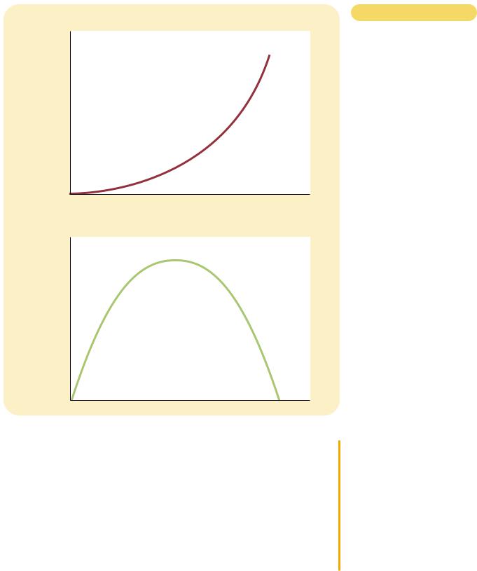
Figure 8-7 summarizes these results. In panel (a) we see that as the size of a tax increases, its deadweight loss quickly gets larger. By contrast, panel (b) shows that tax revenue first rises with the size of the tax; but then, as the tax gets larger, the market shrinks so much that tax revenue starts to fall.
CASE STUDY THE LAFFER CURVE AND
SUPPLY-SIDE ECONOMICS
One day in 1974, economist Arthur Laffer sat in a Washington restaurant with some prominent journalists and politicians. He took out a napkin and drew a figure on it to show how tax rates affect tax revenue. It looked much like panel
(b) of our Figure 8-7. Laffer then suggested that the United States was on the downward-sloping side of this curve. Tax rates were so high, he argued, that reducing them would actually raise tax revenue.
Most economists were skeptical of Laffer’s suggestion. The idea that a cut in tax rates could raise tax revenue was correct as a matter of economic theory, but there was more doubt about whether it would do so in practice. There was little evidence for Laffer’s view that U.S. tax rates had in fact reached such extreme levels.
Nonetheless, the Laffer curve (as it became known) captured the imagination of Ronald Reagan. David Stockman, budget director in the first Reagan administration, offers the following story:
[Reagan] had once been on the Laffer curve himself. “I came into the Big Money making pictures during World War II,” he would always say. At that time the wartime income surtax hit 90 percent. “You could only make four pictures and then you were in the top bracket,” he would continue. “So we all quit working after four pictures and went off to the country.” High tax rates caused less work. Low tax rates caused more. His experience proved it.
When Reagan ran for president in 1980, he made cutting taxes part of his platform. Reagan argued that taxes were so high that they were discouraging hard work. He argued that lower taxes would give people the proper incentive to work, which would raise economic well-being and perhaps even tax revenue. Because the cut in tax rates was intended to encourage people to increase the quantity of labor they supplied, the views of Laffer and Reagan became known as supply-side economics.
Subsequent history failed to confirm Laffer’s conjecture that lower tax rates would raise tax revenue. When Reagan cut taxes after he was elected, the result
Deadweight
Loss
CHAPTER 8
(a) Deadweight Loss
APPLICATION: THE COSTS OF TAXATION |
173 |
Figur e 8-7
HOW DEADWEIGHT LOSS AND
TAX REVENUE VARY WITH THE
SIZE OF A TAX. Panel (a) shows that as the size of a tax grows larger, the deadweight loss grows larger. Panel (b) shows that tax revenue first rises, then falls. This relationship is sometimes called the Laffer curve.
0 |
Tax Size |
(b) Revenue (the Laffer curve)
Tax
Revenue
0 |
Tax Size |
was less tax revenue, not more. Revenue from personal income taxes (per person, adjusted for inflation) fell by 9 percent from 1980 to 1984, even though average income (per person, adjusted for inflation) grew by 4 percent over this period. The tax cut, together with policymakers’ unwillingness to restrain spending, began a long period during which the government spent more than it collected in taxes. Throughout Reagan’s two terms in office, and for many years thereafter, the government ran large budget deficits.
Yet Laffer’s argument is not completely without merit. Although an overall cut in tax rates normally reduces revenue, some taxpayers at some times may be on the wrong side of the Laffer curve. In the 1980s, tax revenue collected from the richest Americans, who face the highest tax rates, did rise when their taxes were cut. The idea that cutting taxes can raise revenue may be correct if applied to

174 |
PART THREE SUPPLY AND DEMAND II: MARKETS AND WELFARE |
|
|
|
|
IN THE NEWS
How to Be Master of the Universe
are known as “God games,” a player assumes total control of a city, a country, or even a galaxy, deciding everything from
One thing these games have in common: Success requires economic growth, and that can only be achieved by keeping taxes low. Tax rates range from the edenic zero to the punitive 80%. With the proceeds of these taxes the player must build costly military or police forces and the infrastructure to support economic and technological advancement.
Why not simply keep taxes high and meet all the “societal needs” a despot could want? Because . . . keeping taxes high leads the population to produce less. As tax rates increase there is, at first, no easily discernable effect on the populace, except perhaps a few frowns and grumbles. But as soon as taxes reach a certain point—10% in some games, 20% in others—citizens begin to revolt. . . .
In games covering a single city, citizens vote with their feet and begin leaving town. No new jobs are created, and
vibrant downtown areas are left little traffic but plenty of crime. Tax that approach 50% or more accelthe trend. . . .
the state or galaxy games, similar apply. During times of great military or bursts of government contax rates can be increased for of years without too much to the populace, and revenues
do increase from the previous year. The government can simply buy what it needs from increased revenue. But a long war or government building program creates problems in “growing the economy” if tax rates are too high. Production slumps. The busy empire builder finds that his starships are harder to produce. Before long a once mighty empire is tottering on the brink of collapse and the ruler is deposed. The wise ruler keeps taxes as low as possible consistent with enough guns and roads to keep the country safe from a takeover by the enemy. . . .
Who says kids are wasting their time playing computers games?
SOURCE: The Wall Street Journal, May 5, 1999, p. A22.
those taxpayers facing the highest tax rates. In addition, Laffer’s argument may be more plausible when applied to other countries, where tax rates are much higher than in the United States. In Sweden in the early 1980s, for instance, the typical worker faced a marginal tax rate of about 80 percent. Such a high tax rate provides a substantial disincentive to work. Studies have suggested that Sweden would indeed have raised more tax revenue if it had lowered its tax rates.
These ideas arise frequently in political debate. When Bill Clinton moved into the White House in 1993, he increased the federal income tax rates on highincome taxpayers to about 40 percent. Some economists criticized the policy, arguing that the plan would not yield as much revenue as the Clinton administration estimated. They claimed that the administration did not fully take into

CHAPTER 8 APPLICATION: THE COSTS OF TAXATION |
175 |
account how taxes alter behavior. Conversely, when Bob Dole challenged Bill Clinton in the election of 1996, Dole proposed cutting personal income taxes. Although Dole rejected the idea that tax cuts would completely pay for themselves, he did claim that 28 percent of the tax cut would be recouped because lower tax rates would lead to more rapid economic growth. Economists debated whether Dole’s 28 percent projection was reasonable, excessively optimistic, or (as Laffer might suggest) excessively pessimistic.
Policymakers disagree about these issues in part because they disagree about the size of the relevant elasticities. The more elastic that supply and demand are in any market, the more taxes in that market distort behavior, and the more likely it is that a tax cut will raise tax revenue. There is no debate, however, about the general lesson: How much revenue the government gains or loses from a tax change cannot be computed just by looking at tax rates. It also depends on how the tax change affects people’s behavior.
QUICK QUIZ: If the government doubles the tax on gasoline, can you be sure that revenue from the gasoline tax will rise? Can you be sure that the deadweight loss from the gasoline tax will rise? Explain.
CONCLUSION
Taxes, Oliver Wendell Holmes once said, are the price we pay for a civilized society. Indeed, our society cannot exist without some form of taxes. We all expect the government to provide certain services, such as roads, parks, police, and national defense. These public services require tax revenue.
This chapter has shed some light on how high the price of civilized society can be. One of the Ten Principles of Economics discussed in Chapter 1 is that markets are usually a good way to organize economic activity. When the government imposes taxes on buyers or sellers of a good, however, society loses some of the benefits of market efficiency. Taxes are costly to market participants not only because taxes transfer resources from those participants to the government, but also because they alter incentives and distort market outcomes.
Summar y
A tax on a good reduces the welfare of buyers and sellers of the good, and the reduction in consumer and producer surplus usually exceeds the revenue raised by the government. The fall in total surplus—the sum of consumer surplus, producer surplus, and tax revenue— is called the deadweight loss of the tax.
Taxes have deadweight losses because they cause buyers to consume less and sellers to produce less, and this change in behavior shrinks the size of the market
below the level that maximizes total surplus. Because the elasticities of supply and demand measure how much market participants respond to market conditions, larger elasticities imply larger deadweight losses.
As a tax grows larger, it distorts incentives more, and its deadweight loss grows larger. Tax revenue first rises with the size of a tax. Eventually, however, a larger tax reduces tax revenue because it reduces the size of the market.

176 |
PART THREE SUPPLY AND DEMAND II: MARKETS AND WELFARE |
Key Concepts
deadweight loss, p. 165
1.What happens to consumer and the sale of a good is taxed? How consumer and producer surplus revenue? Explain.
2.Draw a supply-and-demand sale of the good. Show the tax revenue.
of supply and demand affect the a tax? Why do they have this effect?
disagree about whether labor taxes deadweight losses?
deadweight loss and tax revenue
Problems and Applications
1.The market for pizza is characterized by a downwardsloping demand curve and an upward-sloping supply curve.
a.Draw the competitive market equilibrium. Label the price, quantity, consumer surplus, and producer surplus. Is there any deadweight loss? Explain.
b.Suppose that the government forces each pizzeria to pay a $1 tax on each pizza sold. Illustrate the effect of this tax on the pizza market, being sure to label the consumer surplus, producer surplus, government revenue, and deadweight loss. How does each area compare to the pre-tax case?
c.If the tax were removed, pizza eaters and sellers would be better off, but the government would lose tax revenue. Suppose that consumers and producers voluntarily transferred some of their gains to the government. Could all parties (including the government) be better off than they were with a tax? Explain using the labeled areas in your graph.
2.Evaluate the following two statements. Do you agree? Why or why not?
a.“If the government taxes land, wealthy landowners will pass the tax on to their poorer renters.”
b.“If the government taxes apartment buildings, wealthy landlords will pass the tax on to their poorer renters.”
3.Evaluate the following two statements. Do you agree? Why or why not?
a.“A tax that has no deadweight loss cannot raise any revenue for the government.”
b.“A tax that raises no revenue for the government cannot have any deadweight loss.”
4.Consider the market for rubber bands.
a.If this market has very elastic supply and very inelastic demand, how would the burden of a tax on rubber bands be shared between consumers and producers? Use the tools of consumer surplus and producer surplus in your answer.
b.If this market has very inelastic supply and very elastic demand, how would the burden of a tax on rubber bands be shared between consumers and producers? Contrast your answer with your answer to part (a).
5.Suppose that the government imposes a tax on heating oil.
a.Would the deadweight loss from this tax likely be greater in the first year after it is imposed or in the fifth year? Explain.
b.Would the revenue collected from this tax likely be greater in the first year after it is imposed or in the fifth year? Explain.
6.After economics class one day, your friend suggests that taxing food would be a good way to raise revenue because the demand for food is quite inelastic. In what sense is taxing food a “good” way to raise revenue? In what sense is it not a “good” way to raise revenue?