

7 Content of the report
Laboratory work № 4-3
I. Homework
(answer on a control question from p. 18).
…
II. Laboratory work № 4-3 implementation protocol.
1) Topic:
DETERMINATION of DAMPED OSCILLATIONS PARAMETERS.
2) Goal: Studying key parameters and method of description for damped oscillations of mechanical systems
3) Scheme of laboratory’s research facility:
|
|
1 – physical pendulum; 2 – moving connector; 3 – plate; 4 – ruler.
|

4) Table of measuring instruments:
|
№ |
Name |
Type |
Serial № |
Grid limit |
Grid unit |
Accuracy class |
|
1. |
Stopwatch |
УXЛ-42 |
|
99,99 |
0,01 sec |
0,01 sec |
|
2. |
Ruler |
|
|
1000 mm |
1mm |
1mm |
5) Equations for calculation:
1. Statistical absolute error for conditional period:
![]() ,
,
where =0,95 – confidence probability; n=5 – number of measurements; t 0,95 ; 5= 2,77 – Student’s coefficient.
2. Average value of damping coefficient:
<β>=1/<τ>,
where < τ> – average value of relaxation time.
3. Average value of logarithmic decay decrement:
<δ> = <β>·<Т>,
where <Т> – average value of conventional period.
4. Cyclic frequency of damped oscillations:
<ω>. = 2π/<Т>.
5. Quality factor:
<Q>=π·<Ne>,
where <Ne> - average value of number of oscillations at which amplitude decreases in e times.
6. Equation of physical pendulum damped oscillations:
x(t) = A0 e–<β>·t cos <ω>t,
where x – displacement of pendulum; A0 – initial amplitude.
6) Table of measurements
|
№ |
τi, s |
Nei |
Ti, s |
ΔTi, c |
(ΔTi)2, c2 |
|
1. |
|
|
|
|
|
|
2. |
|
|
|
|
|
|
3. |
|
|
|
|
|
|
4. |
|
|
|
|
|
|
5. |
|
|
|
|
|
|
|
<τ>= … |
<Ne > = … |
<T> = … |
Σ(ΔTi)2= |
… |
7) Quantities calculation:
…
8) Final results:
1.
T=(
<T>±ΔT)α
= ( …
± …
)0.95
s,
![]() = … %;
= … %;
2. x(t) = …e–…t cos(…t +…) m;
3. <δ> =…;
4. <Q>=… .
9) Conclusion:
(Compare obtained value of conventional period with eigenperiod defined in previous laboratory work № 4-1).
10) Work done by: Work checked by:
WORK 4-6
EXPLORING of FORCED OSCILLATIONS in SERIES RLC-CIRCUIT
1 Goal of the work:
1. Studying of dependencies of current and voltage on capacitor in the RLC-circuit from ratio of driving frequency and circuit eigenfrequency.
2. Studying resonance phenomena in AC circuit.
2 Main concepts
Forced (or driven) oscillations are the continuous oscillations of oscillatory system, when the system experiences action of external periodical force.
I
Figure 5 –
Series RLC-circuit.

If we connect in series (Fig. 5) capacitor, resistor, inductor and external source of periodical alternating EMF (generator), the oscillations, which will appear in such circuit, will be forced (or driven).
Let’s consider oscillations of current and voltages in series RLC-circuit driven by external EMF varying under harmonic law:
|
=mcos(Ωt+φ0), |
(46) |
|
|
|
here m – external EMF amplitude, φ0 – external EMF’s initial phase, Ω – external EMF’s cyclic frequency (driving cyclic frequency).
Now let’s apply second Kirchhoff’s rule to the given RLC-circuit:
|
uR + uC = BACK + mcos(Ωt+φ0), |
(47) |
here uR=iR – the voltage on resistor, uC=q/C – voltage on capacitor. Produced by inductor the back EMF eBACK=–L(di/dt) we obtain from self-induction law. Taking into account all mentioned above, let’s rearrange equation (47) as
|
|
(48) |
Differentiation of (28) and division it on L gives
|
|
(49) |
here i
=
![]() .
Introducing notations β =
.
Introducing notations β =![]() and
and![]() we’ll
have
we’ll
have
|
|
(50) |
This second order linear non-homogeneous differential equation is differential equation of driven oscillations. Its solution
|
i(t) = I0e-βtcos(ωt + φ0) + Imcos(Ωt + φ0+). |
(51) |
First term in (51) represents natural damped oscillations of current in the circuit with frequency ω (40), which quite fast decay. So further we’ll deal only with second term of (51):
|
i (t) =Im cos(Ωt +) |
(52) |
called the steady state solution of driven oscillations differential equation. As it seen from (46) and (52) current varies under the same law with the same frequency Ω, as the driving EMF do, but with the phase difference DF.
Let's choose a current's initial phase equal to zero φ0=0, and denote its phase lead as (or phase lag of external EMF –) we’ll have
|
i (t) =Im cosΩt ; |
(53) |
|
(t) =mcos(Ωt–Ф), |
(54) |
where Im is the amplitude of current, which has to be determined.
In order to determine current amplitude and the phase lead , let’s substitute instantaneous value of current (53) in (47) and consider each term of obtained equation:
1. Voltage on inductor uL. With the assumption that inductor has no active resistance, the voltage uL is equal to self-induction (back) EMF with opposite sign:
|
uL= |
(55) |
here UmL=ImΩL=ImXL – amplitude of voltage on inductor and
XL=ΩL – inductive reactance.
2. Voltage on resistor uR.
|
uR=iR=UmR cosΩt , |
(56) |
here ImR=UmR – amplitude of voltage on resistor and
R – resistance of resistor.
3. Voltage
on capacitor uC.
From definition of current i
=
![]() ,
thendq=idt
and
,
thendq=idt
and
|
|
(57) |
Thus from definition of electrocapacity
|
uC
= |
(58) |
where UmC
=![]() =
Im
XC
– amplitude of voltage on capacitor and
=
Im
XC
– amplitude of voltage on capacitor and
XC = 1 / C – capacitive reactance. Both XL and XC measured in Ohms.
Substituting (55), (56) and (58) in (47) we’ll have
|
UmL
cos(Ωt
+ |
(59) |
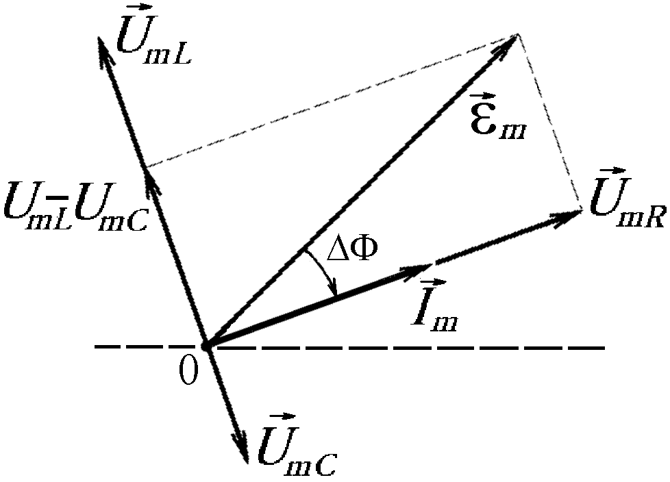
As seen in (59) the external EMF is equal to the sum of three harmonic oscillations with same frequency but different initial phases. In order to sum these oscillations let’s usevector diagram method.In this method each oscillation is being graphically represented as a vector that revolved around some axis with angular velocity equal to the driving cyclic frequency Ω. Length of each vector equals to amplitude of the individual oscillation. The angles between these vectors equal to phase difference that individual oscillations have with respect to each other. Vector representation of (59) shown on a Fig.6.
|
|
|
|
|
Figure 6 – Vector diagram of voltages on RLC-circuit’s elements at low frequency Ω<ω0 (current has a phase lead relative to an external EMF). |
|
Figure 7 – Instantaneous values of current and EMF in RLC-circuit at low frequency Ω<ω0 (current has a phase lead relative to an external EMF). |


Simple geometry gives:
![]() or
or
![]() ,
so
,
so
|
|
(60) |
 .
.This equation is analogue of Ohm’s law for DC homogeneous circuit unit, if to introduce the impedance:
|
|
(61) |
here XC –XL is the reactance of the circuit, R – resistance. Phase lead of current relative to an EMF (see Fig.6):
|
|
(62) |
|
|
|
|
|
Figure 8 – Vector diagram of voltages on RLC-circuit’s elements at high frequency Ω>ω0 (current has a phase lag DF relative to an external EMF).
|
|
Figure 9 – Instantaneous values of current and EMF in RLC-circuit at high frequency Ω>ω0 (current has a phase lag relative to an external EMF). |

Let’s analyze obtained equations. Obviously that change of driving frequency Ω will lead to change of current amplitude Im. On Fig. 10 represented plot of Im versus Ω. From equation (60) follows that:
a) If Ω = 0, then XC and Im = 0. Increasing of Ω leads to increasing of a current;
At low frequency Ω<<ω0 current is limited by capacitance reactance XC>>XL :
 and
and
![]() (see Fig.6 and 7).
(see Fig.6 and 7).
b) At high frequency Ω>>ω0 current is limited by inductive reactance XC<<XL :
 and
and
![]() (see Fig.8 and 9).
(see Fig.8 and 9).
Increasing of driving frequency Ω leads to further decreasing of a current.
c) When the UmC =UmL (voltage resonance), then current’s amplitude has a maximum:
![]() and
and
![]() (see Fig.10 and 11).
(see Fig.10 and 11).
The resonance frequency we find from resonance condition for reactance XC =XL :
![]() ,
so
,
so
![]() or
or
![]() .
.
So we see that Ω RES= ω0.
|
|
|
|
|
Figure 10 – Vector diagram of voltages on RLC-circuit’s elements at resonance Ω = ω0 (current synphase to an external EMF). |
|
Figure 11 – Instantaneous values of current and EMF in RLC-circuit at resonance Ω = ω0 (current synphase to an external EMF). |


Resonance is a fast increasing of amplitude of oscillations when the driving mechanism’s frequency approach to eigenfrequency. Then circuit’s impedance equal to it active resistance and phase difference Ф between driving EMF and current equal zero. Obviously that maximal value of current depends only on active resistance of the circuit. On a Fig. 12 represented current’s amplitude in the circuit for different values of its resistance (quality factor).
At
resonance, forces of electric field, created by EMF source, tend to
accelerate motion of charges. The
amplitude would be increasing to infinity during the time of period
if there was no active resistance in the circuit. In
the real-world circuit increasing of a current leads to increasing of
energy losses. Amplitude of current will approach its steady-state
value when these losses will be equal to work done by the source’s
electric field forces. Phase difference Ф
between current and EMF isn’t equal zero when driving frequency
doesn’t equal to eigenfrequency. In this case, at o
Figure 12 –
Resonant curves: amplitude of current versus driving frequency plot
for different values of resistance and quality factor: R1<R2<R3;
Q1>Q2>Q3.
At resonance the circuit consume a minimum energy from the source. Stored energy of electric field WC=CUmC2/2 completely transforms into energy of magnetic field WL=LIm2/2 and vice versa, as in the case of harmonic oscillations. Source’s energy spent only to compensate energy losses in the circuit. Instantaneous value of a power loss can be determined as:
P(t)
= i(t)u(t)
= ImcosΩt
RImcosΩt
=
![]() Rcos2Ωt.
Rcos2Ωt.
Circuit’s energy loss during the period
![]() ,
,
as
![]()
Resonant properties of RLC-circuit can be characterized by the quality factor :
![]()
One of physical senses of a quality factor is the ratio of energy stored in the circuit to energy dissipated at resonance:
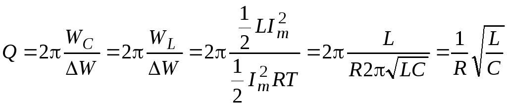 .
.
From voltage resonance condition we have equality of UmL and UmC magnitudes, but, they are in antiphase, so at any instant their sum equals zero:
UmL
= UmC
= Im![]() =
=![]() =m
=m![]() =mQ.
=mQ.
Thus we get another physical sense of quality factor, according which quality shows in how many times the inductance voltage amplitude or capacitance voltage amplitude at resonance greater than driving EMF amplitude:
![]()
 Figure
13 – Amplitude – frequency
characteristics: capacitance, inductance voltages and current’s
amplitudes versus driving frequency Ω.
Figure
13 – Amplitude – frequency
characteristics: capacitance, inductance voltages and current’s
amplitudes versus driving frequency Ω.
For small
active resistance, i.e. if R<<![]() ,
Q>>1,
hence UmL=UmC>>m.
,
Q>>1,
hence UmL=UmC>>m.
Than higher is quality than clearly and sharply resonance is. This is another physical sense of quality factor :
![]() ,
,
here – full width of resonance at half energy maximum (FWHM).
On the Fig. 12 represented current’s amplitude-frequency characteristics for different values of quality factor. It is visible, that higher quality factor has a narrow FWHM.
As it was mentioned above amplitudes of inductance and capacitance depend on the frequency of driving EMF. Expression for amplitude of voltage on inductor can be written as:
|
UmL=ImΩL= |
(63) |
 .
.
Voltage on
inductor
approaches maximum at frequency ΩL
that is greater then circuit’s resonant frequency ΩRES=ω0.
In order to find ΩL
it is necessary to investigate expression (63) of the maximum, i.e.
solve the equation![]() .
.
Amplitude of voltage on capacitor equals
|
UmC= |
(64) |
 .
.It approaches maximum at frequency ΩC that is smaller than ΩRES=ω0.
As it seen from Fig. 13 at ΩRES=ω0 amplitudes UmCRES and UmLRES are numerically equal but not maximal !! Difference of frequencies ΩL – ΩC is smaller than greater quality of the circuit is. At high quality factor ΩC ≈ ΩRES=ω0 ≈ ΩL .