

6) Table of measurements
m = … kg; Δm =0,001 kg; l = … m; Δl = 0,001 m;
|
№ |
ti, s |
Ti, s |
ΔTi, s |
(ΔTi)2, s2 |
|
1. |
|
|
|
|
|
2. |
|
|
|
|
|
3. |
|
|
|
|
|
4. |
|
|
|
|
|
5. |
|
|
|
|
|
average value <T>= |
… |
|
… | |
7) Data processing:
…
8) Final results:
1.
T=(
<T> ± ΔT)α
= ( …
± …
)0.95
s,
 = … %.
2. x(t) = … cos(…t +…) m;
3.
JEXP
= (<
J>
± ΔJ)α
=
( …
± …
)0.95
kg·m2,
![]() =
… %;
=
… %;
4. JTHEOR = … kg·m2;
5. l eq = … m.
9) Conclusion:
(Compare moment of inertia defined experimentally by formula (22) with that of defined by theoretical calculation by formula (23)).
10) Work done by: Work checked by:
WORK 4-3
DETERMINATION of DAMPED OSCILLATIONS PARAMETERS
1 Goal of the work:
Studying key parameters and method of description for damped oscillations of mechanical systems.
2 Main concepts
Real-world oscillatory systems experience different kind of resistances. They loose its energy and with no external energy supply they stop after some finite interval of time. Damped oscillations are such type of free oscillations, which energy decreases with time.
Mechanical energy of oscillatory system gradually decreases transforming into heat. This process called energy dissipation, and such system – dissipative system.
Besides the restoring (quasi-elastic) force (9) that acts in natural oscillatory systems, in the free linear oscillatory systems a drag force acts:
FDRAG = – rυ, (36)
where υ – velocity of pendulum’s moving; r – drag coefficient. “Minus” on the right hand side of (36) means that the drag force always acts in the opposite direction of the velocity.
Thus, for two forces (9) and (36) Newton’s second law for linear damped oscillations will be
ma = —kx—rυ.
In scalars, substituting acceleration of motion a=d2x/dt2 and velocity of motion υ = dx/dt and obtain
![]() ,
,
where m – mass of oscillator (a body or a system of oscillating bodies).
Now let’s rearrange this equation and obtain an equation of damped oscillator in differential view:
![]() ,
(37)
,
(37)
here we introduce designations of variables:
![]() ,
,
![]() .
.
Solution for this differential equation will be the dependence of displacement x from time t, which is termed equations of damped oscillations :
x(t)=A0e–βtcos(ωt+φ01) or x(t)= A0e–βtsin(ωt+φ02), (38)
The basic parameters of damping oscillations are:
damping coefficient (damping factor)
![]() (39)
(39)
and cyclic frequency of damped oscillations
![]() (40)
(40)
h
 Figure
2 – The
underdamping oscillations.
Figure
2 – The
underdamping oscillations.
On the Fig. 2 represented plots of amplitude versus time (dashed line) and displacement versus time (solid line) dependencies.
Damped oscillations are non-periodic: values of oscillating physical quantities (such as displacement, velocity, acceleration) never repeat in damped oscillations process. That is why we can’t use concepts of period and frequency in the way that it been done for periodic (undamped) oscillations.
Conventional period of damped oscillations is such interval of time between to serial states of oscillating system at which oscillating physical quantities vary in the same direction, decreasing or increasing their magnitudes.
Knowing
that
![]() and ω=2π/T
, obtain
and ω=2π/T
, obtain
![]() .
(41)
.
(41)
T
Figure 3 –
Different modes of damping: harmonic;
underdamping;
critical; overdamping.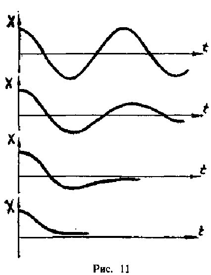
There are different modes of oscillating systems with respect to value of damping coefficient (see Fig.3):
a) β = 0, so r = 0, T=2π/ω0=T0 – harmonic oscillations;
b)
β<ω0,
ω02–β2>0,
![]() –
almost periodic underdamping
mode;
–
almost periodic underdamping
mode;
c) β = ω0, ω02–β2=0, T→ ∞ – aperiodic critical mode;
d) β>ω0, ω02–β2<0, T is imaginary – overdamping mode.
Decay decrement is a ratio of two serial amplitudes of the same sign At and At+T separated in time from each other by the period T:
 .
.
Logarithmic decay decrement is a natural logarithm of this ratio:
![]() .
(42)
.
(42)
In practical calculations, for small damping, it is usually suggested that δ = βT0, where T0 – period of undamped oscillations of the system.
Denoting a τ – relaxation time as interval of time over which the amplitude of oscillations decreases in e times (e = 2.7183 – is the base of natural logarithm), we can write:
![]() .
.
Hence, βτ = 1, or
![]() .
(43)
.
(43)
Thus, for meaning (physical sense) the damping coefficient β it is inversely proportional time over which amplitude of oscillations decreases in e = 2.7 times.
By the time τ system makes Ne = τ/T oscillations (relaxation number), so, taking into account (42) and (43) we’ll have
![]() .
(44)
.
(44)
So, for meaning (physical sense) the logarithmic decay decrement it is inversely proportional to number of oscillations producing by the time over which amplitude of oscillations decreases in e = 2.7 times.
Quality factor of a system is a ratio of coefficients from equation of damped oscillator (37):
![]() .
.
Taking into account previous equations we obtain
![]() .
(45)
.
(45)
Thus, for meaning (physical sense) the quality factor it is proportional to the number of oscillations Ne done by a system by the time τ over which amplitude of oscillations decreases in e = 2.7 times.