

|
|
|
|
|
CURRENT STATE OF |
THE |
HUMAN GENETIC MAP |
|
|
195 |
|||
TABLE |
6.1 |
Genetic and Physical Map Lengths of the Human Chromosomes |
|
|
|
|
|
||||||
|
|
|
|
|
|
|
|
|
|
|
|
|
|
|
|
|
|
|
|
|
|
|
Genetic Size |
|
|
|
|
|
|
|
|
|
|
|
|
|
|
|
|
|
|
|
|
|
Physical |
|
Sex |
|
|
|
|
|
|
|
|
Chromosome |
a |
Size (Mb) |
Averaged |
cM/Mb |
Female |
cM/Mb |
Male |
cM/Mb |
|
|
|||
|
|
|
|||||||||||
|
|
|
|
|
|
|
|
|
|
|
|||
|
1 |
|
263 |
292.7 |
1.11 |
|
358.2 |
1.36 |
220.3 |
0.84 |
|||
|
2 |
|
255 |
277.0 |
1.09 |
|
324.8 |
1.27 |
210.6 |
0.83 |
|||
|
3 |
|
214 |
233.0 |
1.09 |
|
269.3 |
1.26 |
182.6 |
0.85 |
|||
|
4 |
|
203 |
212.2 |
1.05 |
|
270.7 |
1.33 |
157.2 |
|
0.77 |
||
|
5 |
|
194 |
197.6 |
1.02 |
|
242.1 |
1.25 |
147.2 |
|
0.76 |
||
|
6 |
|
183 |
201.1 |
1.10 |
|
265.0 |
1.45 |
135.2 |
|
0.74 |
||
|
7 |
|
171 |
184.0 |
1.08 |
|
187.2 |
1.09 |
178.1 |
|
1.04 |
||
|
8 |
|
155 |
166.4 |
1.07 |
|
221.0 |
1.43 |
113.1 |
|
0.73 |
||
|
9 |
|
145 |
166.5 |
1.15 |
|
194.5 |
1.34 |
138.5 |
|
0.96 |
||
|
10 |
|
144 |
181.7 |
1.26 |
|
209.7 |
1.46 |
146.1 |
1.01 |
|||
|
11 |
|
144 |
156.1 |
1.08 |
|
180.0 |
1.25 |
121.9 |
|
0.85 |
||
|
12 |
|
143 |
169.1 |
1.18 |
|
211.8 |
1.48 |
126.2 |
|
0.88 |
||
|
13q |
|
98 |
117.5 |
1.20 |
|
132.3 |
1.35 |
97.2 |
|
0.99 |
||
|
14q |
|
93 |
128.6 |
1.38 |
|
154.4 |
1.66 |
103.6 |
|
1.11 |
||
|
15q |
|
89 |
110.2 |
1.24 |
|
131.4 |
1.48 |
91.7 |
|
1.03 |
||
|
16 |
|
98 |
130.8 |
1.33 |
|
|
169.1 |
1.73 |
98.5 |
|
1.01 |
|
|
17 |
|
92 |
128.7 |
1.40 |
|
145.4 |
1.58 |
104.0 |
|
1.13 |
||
|
18 |
|
85 |
123.8 |
1.46 |
|
|
151.3 |
1.78 |
92.7 |
|
1.09 |
|
|
19 |
|
67 |
109.9 |
1.64 |
|
115.0 |
1.72 |
98.0 |
|
1.46 |
||
|
20 |
|
72 |
96.5 |
1.34 |
|
|
120.3 |
1.67 |
73.3 |
|
1.02 |
|
|
21q |
|
39 |
59.6 |
1.53 |
|
|
70.6 |
1.81 |
46.8 |
|
1.20 |
|
|
22q |
|
43 |
58.1 |
1.35 |
|
74.7 |
1.74 |
46.9 |
|
1.09 |
||
|
X |
|
164 |
198.1 |
1.21 |
|
198.1 |
1.21 |
|
|
|
||
|
|
|
|
|
|
|
|
|
|
|
|
||
Source: |
Adapted from Dib et al. (1996). |
|
|
|
|
|
|
|
|
|
|
||
a Only the long arm is shown for five chromosomes in which the short arm consists largely |
of |
tandemly repeat- |
|
|
|
|
|||||||
ing ribosomal DNA. The approximate full length of these chromosomes are given in parentheses. |
|
|
|
|
|
|
|||||||
CURRENT STATE OF THE HUMAN GENETIC MAP |
|
|
|
|
|
||||
Several |
major |
efforts to make genetic maps of the human |
genome have occurred |
during |
|||||
the past few years, and recent emphasis has been on merging these efforts to forge con- |
|||||||||
sensus maps. A few examples of the status of these maps several years ago are given in |
|||||||||
Figure 6.29 |
a |
and |
b . These are sex-averaged |
maps |
because they |
have |
a larger density of |
||
markers. |
The |
ideal framework map will have markers |
spaced |
uniformly |
at |
distances |
|||
around 3 to 5 cM, since this is the most efficient sort of map to use to |
try to find addi- |
||||||||
tional markers or disease genes with current technology. On this basis the map shown for |
|||||||||
chromosome 21 is quite mature, while the map for chromosome 20, a much less studied |
|||||||||
chromosome, is still relatively immature. Chromosome 21 is completely covered (except |
|||||||||
for the rDNA-containing short arm) with relatively uniform markers; in contrast, chromo- |
|||||||||
some 20 has several regions where the genetic resolution is much worse than 5 cM. The |
|||||||||
current |
status |
of |
the maps |
can only be summarized highly |
schematically, |
as |
shown in |
||
Figure 6.29 |
c . Here 2335 positions defined by 5264 markers are plotted. On average, this |
||||||||
is almost 1 position per cM. |
|
|
|
|
|
|
|||

196 GENETIC ANALYSIS
Figure 6.29 |
Genetic maps |
of |
human |
chromo- |
||||
somes. |
(a,b) |
|
Status of sex-averaged maps |
of |
chro- |
|||
mosomes |
20 |
and |
21 |
several |
years ago. |
(c) |
||
Schematic |
summary |
of |
current |
genetic |
map |
(from |
|
|
Dib et al., 1996).

GENETICS IN THE PSEUDOAUTOSOMAL REGION |
197 |
Figure 6.29 (Continued)
The physical lengths of the human chromosomes are estimated to range from 50 Mb for chromosome 21, the smallest, to 263 Mb for chromosome 1, the largest. Table 6.1 summarizes these values and compares them with the genetic lengths, seen separately from male and female meioses. Several interesting generalizations emerge from an inspection of Table 6.1. The average recombination frequency per unit length (cM per Mb) varies over a broad range from 0.73 to 1.46 for male meioses and 1.09 to 1.81 for female meioses. Smaller chromosomes tend to have proportionally greater genetic lengths, but
this effect is by no means uniform. Recombination along the X chromosome (seen only in females) is markedly suppressed compared with autosomal recombination.
Leaving the details of the genetic map aside, the current version is an extremely useful
tool for finding genes on almost every chromosome. As this |
map |
is used |
on a broader |
||
range |
of individuals, we should start to |
be able to pinpoint potential |
recombination hot |
||
spots |
and explore whether these are |
common throughout |
the |
human |
population or |
whether some or all of them are allelic variants. The present map is already a landmark accomplishment in human biology.
GENETICS IN THE PSEUDOAUTOSOMAL REGION
Meiotic recombination in the male produces a special situation. The male has only one X and one Y chromosome. These must segregate properly to daughter cells. They must pair with each other in meiotic metaphase, and by analogy with the autosomes, one expects that meiotic recombination will be an obligatory event in proper chromosome segregation.

198 GENETIC ANALYSIS
Figure 6.30 Pairing between the short arms of the X and Y chromosomes in male meiosis.
The problem |
this raises is that the X and Y are very different in size, |
and much of these |
two chromosomes appear to share little homology. How then does recombination occur |
||
between them? It turns out that there are at least two regions of the Y chromosome that |
||
share close |
enough of the X to allow recombination. These are called |
pseudoautosomal |
regions, |
for reasons that will become apparent momentarily. |
|
The major psuedoautosomal region of the Y chromosome is located at the tip of the |
||
short arm. It is about 2.5 Mb in length and corresponds closely in DNA sequence with the |
||
2.5 Mb short arm terminus of the X chromosome. These two regions are observed to pair |
||
up during meiosis, and recombination presumably must occur in this region (Fig. 6.30). If |
||
we imagine an average of 0.5 crossovers per cell division, this is a very high recombina- |
||
tion rate indeed compared to a typical autosomal region. |
|
|
Since the Y chromosome confers a male phenotype, somewhere on this chromosome |
||
must lie a gene or genes responsible for male sex determination. We know that this region |
||
lies below the pseudoautomal boundary, a place about 2.5 Mb from the short term telo- |
||
mere. Below |
this boundary, genes appear to be sex linked because, by definition, these |
|
genes must not be able to separate away from the sex determination region in meiosis. A |
||
genetic map of the pseudoautomal region of the Y chromosome is shown in Figure 6.31. |
||
There is a |
gradient of recombination probability across the region. Near the p |
telomere, |
all genes will show 50% recombination with the sex-determining region because of the obligatory recombination event during meiosis. Thus these genes appear to be autosomal, even though they are located on a sex chromosome, because like genes on autosomes they
Figure 6.31 Genetic map of the pseudoautosomal region of the X and Y chromosomes.

|
|
|
|
GENETICS IN THE PSEUDOAUTOSOMAL REGION |
199 |
|
have a 50% probability of being inherited with each sex. As one nears the pseudoautoso- |
|
|||||
mal boundary, the recombination frequency of genes with the sex determination region |
|
|||||
approaches |
a more normal value, and these genes appear |
to be almost completely sex |
|
|||
linked. |
|
|
|
|
|
|
Recently data have been obtained that indicate that a second significant pseudoautoso- |
|
|||||
mal region |
may |
lie at |
the extreme ends of the |
long arms |
of the X and Y chromosomes. |
|
About 400 |
kb |
of DNA |
in these regions appears |
to consist |
of homologous sequences, and |
|
a 2% recombination frequency in male meioses between two highly informative loci in these regions has been observed. The significance of DNA pairing and exchange in this region for the overall mechanism of male meiosis is not yet known. It is also of interest to examine whether in female meiosis any or all of the X chromosome regions that are homologous to the pseudoautosomal region of the Y chromosome show anomalous recombination frequencies.
BOX |
6.4 |
|
|
|
|
|
MAPPING FUNCTIONS: ACCOUNTING |
|
|
|
|
|
|
FOR |
MULTIPLE RECOMBINATIONS |
|
|
|
|
|
If |
two markers are not close, there is |
a |
significant |
chance |
that multiple |
DNA |
crossovers may occur between them in a particular meiosis. What one observes experi- |
|
|||||
mentally is the net probability of recombination. A more accurate measure of genetic |
|
|||||
distance will be the average number of crossovers that has occurred between the two |
|
|||||
markers. We need to correct for the occurrence of multiple crossovers in order to com- |
|
|||||
pute the expected number of crossovers from the observed recombination frequency. |
|
|||||
This is done by using a mapping function. |
|
|
|
|
|
|
|
The various possible recombination events for zero, one, and two crossovers are il- |
|||||
lustrated schematically in Figure 6.32. In each case we are interested in correlating the |
||||||
observed number of recombinations between two distant markers and the actual aver- |
|
|||||
age |
number of crossovers among the DNA strands. In all the examples discussed be- |
|
||||
low it is important to realize that any crossovers that occur between sister chromatids |
||||||
(identical copies of the parental homologs) have no effect on the final numerical re- |
||||||
sults. The simplest case occurs where there are no crossovers between the markers; |
|
|||||
clearly in this case there is no recombination between the markers. Next, consider the |
|
|||||
case |
where there is a single crossover between |
two |
different |
homologs |
(Fig. 6.32 |
b ). |
The |
net result is a 0.5 probability of recombination because half |
of the sister chro- |
||||
matids will have been involved in the crossover and half will not have been. |
|
|||||
|
When two crossovers occur between the markers, the results are much more com- |
|
||||
plex. Three different cases are illustrated in Figure 6.32 |
|
c . Two single crossovers can oc- |
||||
cur, each between a different set of sister chromatids. The net result, shown in the figure, is that all the gametes show recombination between the markers; the recombination frequency is 1.0. There are four discrete ways in which these crossovers can occur. Alternatively, the two crossovers may occur between the same set of sister chromatids. This is a double-crossover event. The net result is no observed recombination between the distant markers. There are four discrete ways in which a double crossover can occur. Note that the net result of the two general cases we have considered thus far is 0.5 recombinant per crossover.
(continued)

200 GENETIC ANALYSIS
BOX 6.4 |
(Continued) |
Figure 6.32 |
Possible crossovers between pairs |
of genetic markers and the resulting meiotic re- |
|||
combination frequencies that would be observed between two |
markers (vertical arrows) flanking |
||||
the region. |
(a) |
No crossovers. |
(b) One crossover. |
(c) Various ways in which two crossovers can |
|
occur. |
|
|
|
|
|
(continued)
|
|
|
|
|
|
|
WHY |
GENETICS NEEDS DNA |
ANALYSIS |
201 |
|||
|
BOX |
6.4 |
(Continued) |
|
|
|
|
|
|
|
|
|
|
|
|
|
|
|
|
|
|
|
|
|
|||
|
The final case we need to consider |
for two crossovers are those |
in |
which |
three of |
|
|
||||||
|
the four paired sister chromatids are |
involved; two are used once |
and one |
is used |
|
|
|||||||
|
twice. There are 12 possible ways in which this can occur. Two representative exam- |
|
|
||||||||||
|
ples are shown in Figure 6.32 |
|
c . Each results in half |
of the DNA strands showing a re- |
|
||||||||
|
combination event between distant markers, and half showing no evidence for such an |
|
|
||||||||||
|
event. Thus, on average, this case yields an observed recombination frequency of 0.5. |
|
|
||||||||||
|
This is also the average for all the cases we have considered except the case where no |
|
|
||||||||||
|
crossovers have occurred at all. It turns out that it is possible to generalize this argu- |
|
|||||||||||
|
ment to any number of crossovers. The observed recombination frequency, |
|
|
|
|
obs |
, is |
||||||
|
|
|
|
|
obs 0.5 (1 P |
0) |
|
|
|
||||
|
where |
P 0 is the fraction of meioses in |
which no |
crossovers occur |
between |
a particular |
|
|
|||||
|
pair of markers. |
|
|
|
|
|
|
|
|
|
|
|
|
|
It is a reasonable approximation to suppose that the number of crossovers between |
|
|
||||||||||
|
two markers will be given by a Poisson distribution, where |
|
|
|
|
represents the mean |
|
||||||
|
number of crossovers that take place in an interval the size of the spacing between the |
|
|
||||||||||
|
markers. The frequency of |
n |
crossovers predicted by the Poisson distribution is |
|
|||||||||
|
|
|
|
|
P n |
n exp( |
) |
|
|
||||
|
|
|
|
|
n ! |
|
|
|
|
||||
|
|
|
|
|
|
|
|
|
|
|
|||
|
and the frequency of zero crossovers is just |
|
P |
0 exp( ). Using this, we can rewrite |
|
||||||||
|
|
|
|
|
obs |
0.5 (1 exp( )) |
|
|
|||||
|
This can easily be rearranged to give |
|
|
as a function of |
|
obs |
: |
|
|||||
|
|
|
|
|
1n(1 2 obs ) |
|
|
||||||
|
The |
parameter |
is the true measure of mapping distance corrected for multiple |
|
|||||||||
|
crossovers. It is the desired mapping function. |
|
|
|
|
|
|
|
|
||||
|
|
|
|
|
|
|
|
|
|
|
|
|
|
WHY GENETICS NEEDS DNA ANALYSIS
In almost all of the preceding discussion, we assumed the ability to determine genotype uniquely from phenotype. We allowed that we could always find heterozygous markers when we needed them, and that there was never any ambiguity in determining the true
genotype from the |
phenotype. This is an ideal situation never quite |
achieved in practice, |
but we can come very close to it by the use of DNA sequences as genetic |
markers. |
|
The simplest |
DNA marker in common use is a two allele polymorphism—a single inher- |
|
ited base pair difference. This is shown schematically in Figure 6.33. From the DNA sequence it is possible to distinguish the two homozygotes from the heterozygote. Earlier, in Chapter 4, we demonstrated how this can be accomplished using allele-specific PCR.
202 GENETIC ANALYSIS
Figure 6.33 Example of a simple RFLP and how it is analyzed by gel electrophoresis and Southern blotting. Such an allele can also be analyzed by PCR or allele-specific PCR, as described
in Chapter 4.
An alternative approach, less general but with great historical precedent, is the examination of restriction fragment length polymorphisms (RFLPs). Such a case is illustrated in Figure 6.33. Where a single-base polymorphism adventitiously lies within the sequence recognized and cleaved by a restriction endonuclease, the polymorphic sequence results in a polymorphic cleavage pattern. All three possible genotypes are distinguishable from the pattern of DNA fragments seen in an appropriate double digest. If this is analyzed by Southern hybridization, it is helpful to have a DNA probe that samples both sides of the polymorphic restriction site,
since this prevents confusion from other possible polymorphisms in the region of interest.
The difficulty with two-allele systems is that there are many cases where they will not be informative in a family linkage study, since too many of the family members will be homozygotes or other noninformative genotypes. These problems are rendered less serious when more alleles are available. For example, two single-site polymorphisms in a re-
gion combine to generate a four-allele system. If these occur at restriction sites, the alleles are both sites cut, one site cut, the other site cut, and no sites cut. Most of the time the resulting DNA lengths will all be distinguishable.
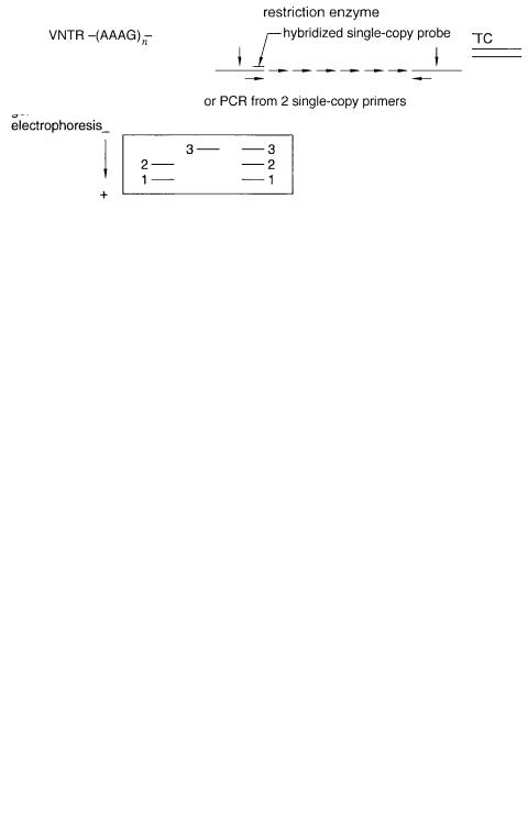
The ideal DNA marker will have a great many easily distinguished alleles. In practice, the most useful markers have turned out to be minisatellites or variable number tandem
repeated sequences (VNTRs). An example is a block like (AAAG) |
n situated between two |
single-copy DNA sequences. This is analyzed by PCR from the two single-copy flanking |
|
regions or by hybridization using a probe from one of the single-copy regions (Figure |
|
6.34). The alleles correspond to the number of repeats. There are a large number of possi- |
|
ble alleles. VNTRs are quite prevalent in the human genome. Many |
of them have a large |
Figure 6.34 Use of PCR to analyze length variations in typical VNTR. In genetics such markers are extremely informative and can be easily found and analyzed.
|
|
DETECTION OF HOMOZYGOUS REGIONS |
|
203 |
|
number of alleles in the actual human population, and thus they are very powerful genetic |
|
|
|||
markers. See, for example, Box 6.5. Most individuals are heterozygous for these alleles, |
|
|
|||
and most parents have different alleles. Thus the particular homologous chromosomes in- |
|
|
|||
herited by an offspring can usually be determined unambiguously. |
|
|
|
||
|
|
|
|
|
|
BOX 6.5 |
|
|
|
|
|
A HIGHLY INFORMATIVE |
POLYMORPHIC MARKER |
|
|
|
|
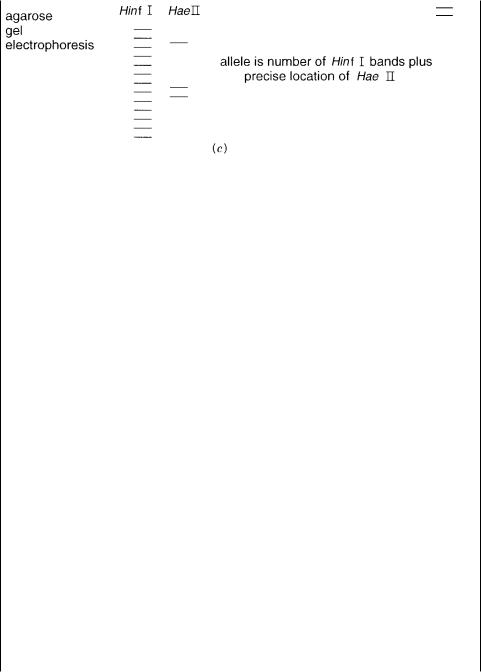
A particularly elegant example of the power of VNTRs is a probe described by Alec |
|
|
|||
Jeffries. This single-copy probe which detects a nearby minisatellite was originally |
|
|
|||
called MS32 by Jeffries (MS means minisatellite). When its location was mapped on |
|
|
|||
the genome, it was found to lie on chromosome 1 and was assigned by official desig- |
|
|
|||
nation D1S8. Here D |
refers to the fact that |
the marker is a DNA sequence, 1 |
means |
|
|
that it is on chromosome 1, S means that it |
is a single copy DNA sequence, |
and 8 |
|
|
|
means that this was the eighth such probe assigned to chromosome 1. The power of |
|
|
|||
D1S8 is illustrated in Figure 6.35. The minisatellite contains a |
Hin f I |
cleavage site |
|||
within each 29 base |
repeat. In addition some repeats contain an internal |
|
Hae |
II cleav- |
|
Figure 6.35 A highly informative genetic marker D1S8 that can be used for personal identity
determinations. |
(a) Repeating DNA structure of the marker. |
(b) PCR production of probes to an- |
|
alyze the marker. |
(c) Typical results observed when the marker is analyzed after separate, partial |
||
Hae |
II and Hin |
f I digestions. |
|
(continued)
204 |
GENETIC ANALYSIS |
|
|
|
|
|
|
|
|
|
BOX |
6.5 |
(Continued) |
|
|
|
|
|
|
|
|
age site. When appropriately chosen PCR primers are used, one can amplify the region |
|
|
||||||||
containing the repeat and radiolabel just one side of |
it. Then |
a partial digestion |
with |
|
||||||
the |
restriction |
enzyme |
Hae |
II or Hin |
f I generates a |
series of DNA bands whose sizes |
|
|||
reflect all of the enzyme-cutting sites within the repeat. This reveals not only the num- |
|
|||||||||
ber of repeats but also the locations of the specific |
|
|
Hae |
II sites. When this information |
|
|||||
is combined, it turns out that there are more than 10 |
|
|
70 |
possible alleles of this sequence. |
|
|||||
Almost every member of the human population (exempting identical twins) would be |
|
|
|
|||||||
expected to have a different genotype here; thus this probe is an ideal one not only for |
|
|
||||||||
genetic analysis but also for personal identification. |
|
|
|
|
|
|
||||
|
By comparing the alleles of D1S8 in males and in sperm samples, the mutation rage |
|
|
|||||||
of this VNTR has been estimated. It is extremely high, about 10 |
|
|
3 per meiosis or 10 |
5 |
||||||
higher than the average rate expected within the human genome. The mechanism be- |
|
|
|
|||||||
lieved to be responsible for this very high mutation rate can be inferred from a detailed |
|
|
||||||||
analysis of the mutant alleles. It turns out that almost all of the mutations arise from |
|
|||||||||
interallelic events, as shown in |
Figure |
6.36. These |
include |
possible |
slippage |
of |
the |
|
||
DNA during DNA synthesis, and unequal sister chromatid exchange. Only 6% of the |
|
|
|
|||||||
observed mutations arise from ordinary meiotic recombination events between homol- |
|
|
|
|||||||
ogous chromosomes. |
|
|
|
|
|
|
|
|
||
Figure 6.36 |
Recombination events that generate diversity in the marker D1S8. |
(a) Intra-allelic |
recombination or polymerase slippage, a very common event. |
(b) Inter-allelic recombination, a |
|
relatively rare event. |
|
|
DETECTION OF HOMOZYGOUS REGIONS
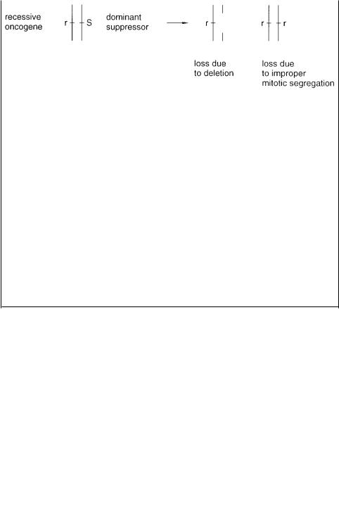
Because the human species is highly outbred, homozygous regions are rare. Such regions can be found, however, by traditional methods or by some of the fairly novel methods that will be described in Chapter 13. Homozygous regions are very useful both in the diagnosis of cancer and in certain types of genetic mapping. The significance of homozygous regions in cancer is
shown in Figure 6.37. Oncogenes are ordinary cellular genes, or foreign genes that under appropriate circumstances can lead to uncontrolled cell growth, that is, to cancer. Quite a few oncogenes have been found to be recessive alleles, ordinarily silenced in the heterozygous
Figure 6.37 Generation of homozygous DNA regions in cancer.