

RELATIONSHIP BETWEEN THE PHYSICAL AND THE GENETIC MAPS |
175 |
Figure 6.10 Effect of a double crossover on the pattern of inheritance at three loci.
tive gene order are illustrated in Figure 6.10. Obviously multiple crossovers between very close loci are improbable, in general, but they are observed, particularly in regions where recombination hotspots abound. Such a double crossover makes more distant loci appear closer than they should.
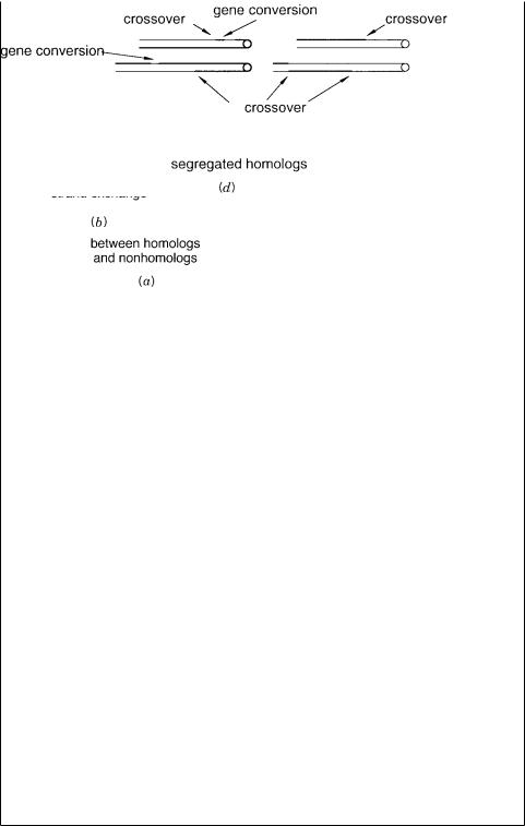
The second genetic complication is gene conversion. Here information from one ho-
mologous chromosome is |
copied onto the corresponding region of another homolog. A |
|
|
schematic |
mechanism is |
given in Figure 6.11, and the consequences for gene order |
are |
shown in |
Figure 6.12. Gene conversion appears to be relatively frequent |
in yeast. |
|
Evidence for human or mammalian gene conversion is much more spotty, but it is generally believed that this process does play a significant role. Gene conversion can make a nearby marker appear to be far away, as shown in Figure 6.12. The exact biological functions of gene conversion remain to be clarified. It potentially forms a mechanism for very rapid evolution, since it allows a change in one copy of a gene to be spread among identi-
cal or nearly identical copies. Gene conversion is also believed to play a role in the sorting out of homologous chromosome pairs prior to crossing over, as described in Box 6.2.
Figure 6.11 |
An example of gene conversion, an event that destroys the usual 1 |
:1 segregation pat- |
tern seen in typical |
Mendelian inheritance. |
|

176 GENETIC ANALYSIS
Figure 6.12 Effect of a gene conversion event on the pattern of inheritance at three loci.
BOX |
6.2 |
|
|
|
|
|
|
|
|
|
|
|
|
TWO-STAGE |
MODEL |
OF |
RECOMBINATION |
|
|
|
|
|
|
|
|||
For recombination to occur, homologous chromosomes must pair up with their DNA |
|||||||||||||
sequences |
aligned. Studies in yeast have led to a rather |
complex |
model for this |
||||||||||
process. The complications occur because DNA sequence similarities or identities oc- |
|||||||||||||
cur |
not only |
between |
the pairs of homologs but also between |
different chromosomes |
|||||||||
as a result of dispersed repeated DNA sequences (see Chapter 14) or dispersed gene |
|||||||||||||
families with similar or identical members. The recombination apparatus in bacteria, |
|||||||||||||
yeast, and presumably all higher organisms has the ability to catalyze sequence simi- |
|||||||||||||
larity searches. In these, a DNA duplex is nicked, and a single-stranded region is ex- |
|||||||||||||
posed and |
covered |
with protein. This is |
then used |
to |
scan |
duplex |
DNA |
by processes |
|||||
we still do not understand very well (see discussion of |
|
|
|
rec A protein in Chapter 14). |
|||||||||
When a close sequence match is found, the single strand can invade the corresponding |
|||||||||||||
duplex and displace its equivalent sequence there. Depending on what happens next, |
|||||||||||||
this |
can |
result either in a gene conversion event in which |
information |
is copied from |
|||||||||
one homolog to the other, a Holliday structure, which may eventually lead to strand re- |
|||||||||||||
arrangement, or in simple displacement of the invading strand and restoration of the |
|||||||||||||
original DNA molecules. |
|
|
|
|
|
|
|
|
|||||
|
Figure 6.13 illustrates some of the stages of these processes in a hypothetical exam- |
||||||||||||
ple of a cell with two different homologous pairs of chromosomes. In meiosis each |
|||||||||||||
chromosome starts as a pair of identical sister chromatids linked at the centromere. |
|||||||||||||
Initial strand exchange (shown as dotted lines between the chromosomes) occurs both |
|||||||||||||
between homologs and between nonhomologs (Fig. 6.13 |
|
|
|
a ). Some gene conversion |
|||||||||
events may result at this stage. As the system is driven toward increasing amounts of |
|||||||||||||
strand exchange (in a manner we do not know), it is clearly much more likely that ho- |
|||||||||||||
mologous pairing dominates (Fig. 6.13 |
|
|
|
b ). Finally, after suitable alignment is reached |
|||||||||
(again, |
judged |
by mechanisms that we have no current knowledge |
about), crossing- |
||||||||||
over |
events |
occur |
(Fig. |
6.13 |
c ), |
and |
the |
homologs segregate to daughter cells (Fig. |
|||||
6.13 d ). Each |
chromosome |
at that point |
consists |
of |
a pair of |
sister |
chromatids that are |
||||||
no longer identical because of the different gene conversion and crossing-over events they have experienced.
(continued)
RELATIONSHIP BETWEEN THE PHYSICAL AND THE GENETIC MAPS |
177 |
BOX 6.2 |
(Continued) |
Figure 6.13 The two-stage model for meiotic recombination. See Box 6.2 for details. (Adapted from Roeder, 1992.)
178 |
|
GENETIC ANALYSIS |
|
|
|
|
|
|
|
|
|||
To distinguish single and multiple crossover events, and gene conversion, large num- |
|
|
|
||||||||||
bers of highly informative loci are |
very helpful. Several features of |
genetic loci |
make |
|
|
|
|||||||
them particularly powerful for mapping. Ideally one has many different alleles, and these |
|
|
|
||||||||||
occur at reasonable frequencies in the population. Where this occurs, there is a very good |
|
|
|
||||||||||
chance that all four parental homologs are distinguishable at the locus because they each |
|
|
|
||||||||||
carry different alleles. A major thrust in human genetics has been the systematic collec- |
|
|
|
||||||||||
tion of such highly informative loci. This will be discussed in a later section. It is also |
|
|
|
||||||||||
helpful to have many offspring in families under study and to have many generations of |
|
|
|
|
|||||||||
family members. Because it is so difficult to satisfy these conditions, human genetics is |
|
|
|
||||||||||
often rendered rather impotent compared with the genetics of more easily manipulatable |
|
|
|
|
|||||||||
experimental organisms. |
|
|
|
|
|
|
|
|
|
||||
POWER |
OF |
MOUSE |
GENETICS |
|
|
|
|
|
|
|
|
||
Mice are among the smallest common mammals. They are relatively inexpensive to main- |
|
|
|
|
|||||||||
tain, have large numbers of offspring, and mature quickly enough to allow many genera- |
|
|
|
|
|||||||||
tions to be examined. However, this alone does not explain why mice form such a power- |
|
|
|
|
|||||||||
ful genetic system. Several reasons exist that make the mouse the preeminent model for |
|
|
|
|
|||||||||
mammalian genetics. First, so much is |
already known about so many mouse |
genes, |
that |
|
|
|
|
||||||
an extensive genetic map already exists. Second, many highly inbred strains of laboratory |
|
|
|
|
|||||||||
mice exist. These tend to be homozygous at most alleles, and thus a description of their |
|
|
|
||||||||||
phenotype and genotype is relatively simple. Also gene transfer and knockout technology |
|
|
|
|
|||||||||
exist for mice. What is |
particularly useful is that rather distant inbred strains of mice can |
|
|
|
|||||||||
be interbred to give at |
least some fertile offspring. This property dramatically simplifies |
|
|
|
|||||||||
the construction of high-resolution genetic maps. Several different sets |
of inbred strains |
|
|
|
|||||||||
can be used. One of |
the earlier |
choices was |
|
Mus |
musculus, |
the common |
laboratory |
|
|||||
mouse, and |
|
|
Mus spretus, |
a distant cousin. |
|
|
|
|
|
|
|
||
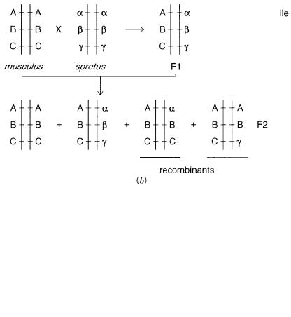
Figure 6.14 illustrates how crosses between |
|
M. musculus |
and |
M. spretus |
generate very |
|
|||||||
useful genetic information. Because these mice are so different, the F1 offspring of a di- |
|
|
|
||||||||||
rect cross tend to be |
heterozygous at almost any locus examined. It turns out that the |
|
|
|
|||||||||
males that result from such a cross are sterile, but the females are fertile. When an F1 |
|
|
|
||||||||||
spretus |
musculus |
female is bred with an |
M. musculus |
|
(a procedure called a |
backcross |
), |
||||||
in most regions of the |
genome the progeny either resemble wild type |
|
|
|
|
M. musculus |
ho- |
||||||
mozygotes, |
or |
F1 |
musculus |
spretus |
heterozygotes. However, |
every time a recombina- |
|
|
|||||
tion event occurs, there is a switch between the homozygous pattern and the heterozygous |
|
|
|
||||||||||
pattern |
(Fig. |
6.14 |
b ). Given the dense set of genetic markers available in these organisms, |
|
|
|
|||||||
the location of many recombination events can be determined in each set of experimental |
|
|
|
|
|||||||||
animals. The result is that one develops and refines genetic maps extremely rapidly. |
|
|
|
|
|||||||||
WEAKNESS |
OF |
HUMAN GENETICS |
|
|
|
|
|
|
|
|
|||
Humans, from |
a |
genetic |
standpoint, are a stark contrast with mice. We have a relatively |
|
|
|
|||||||
long generation time; it precludes the simultaneous availability of large numbers of gen- |
|
|
|
||||||||||
erations. |
Our |
families |
are small; most are far too small for effective genetics. Crosses |
|
|
|
|||||||
cannot be controlled, and there are no inbred strains, only the occasional result of very |
|
|
|
||||||||||
limited inbreeding in particular cultures that promote such practices as marriages between |
|
|
|
|
|||||||||
WEAKNESS OF HUMAN GENETICS |
179 |
Figure 6.14 |
Example of the informativeness of a back cross between two |
distant mouse |
species |
||
M. musculus |
and |
M. spretus. (a) |
Design of the back cross. |
(b) |
Alleles seen for three loci in the par- |
ents and the first (F1) and typical second (F2) generation of offspring, with and without recombination.
cousins. For all of these reasons, the design and execution of prospective genetic experiments is impossible in the human. Instead, one must do retrospective genetic analysis on existing families. Ideally these will consist of family units where at lest three generations are accessible for study. Results from many different families usually must be pooled in order to have enough individuals segregating a trait of interest to allow a statistically significant test of hypotheses about the model for its inheritance. Usually that test is to ask if
the |
trait is linked to any other known trait |
in the genome. This is a very tedious task, as |
we |
will illustrate. However, large numbers of |
ongoing studies use this approach because |
it is the only effective way we have to find a human gene location if the only available information we have is a disease phenotype. If there are animal models for the trait in question, or if one has a hint about the functional defect, one can sometimes cut short a search of the entire genome by focusing on candidate genes. However, these genes still must be examined in linkage studies with human markers because the arrangement of genes in hu-
mans and model organisms, while similar (Fig. 2.24), is not identical.

180 |
GENETIC |
ANALYSIS |
|
|
|
There are several additional major weaknesses that compromise the power of human |
|||||
genetics. In many cases our ability to |
evaluate the phenotype is imprecise. For example, |
||||
in inherited diseases it is not at all uncommon to have imprecise or even incorrect diag- |
|||||
noses. These result in the equivalent of a recombination event as far as genetics is con- |
|||||
cerned, and a few such errors can often |
destroy the chances |
that a search for a gene will |
|||
be successful. A second common problem |
is missing or uncooperative family |
members. |
|||
In such cases the family tree, called |
a |
pedigree, |
is incomplete, and phase or other infor- |
||
mation about the inheritance of a disease trait, or a potential nearby marker, is lost. |
|||||
Homozygosity in key individuals is another frequent problem. As illustrated earlier, this |
|||||
makes it impossible to determine which |
parental homolog in the region of interest has |
||||
been inherited. As genetic markers become denser and more informative, this problem is |
|||||
becoming less severe, but it is by no means uncommon yet. |
|
|
|||
The |
final problem |
that frequently plagues human genetic |
studies is mispaternity. This |
||
is relatively easy to discover by using the highly informative genetic markers currently available. Usually the true parent is not identified; this results in a missing family member for genetic studies.
LINKAGE ANALYSIS IGNORING RECOMBINATION
The statistical analysis of linked inheritance is the tool used for almost all genetic studies in the human. Here we introduce this approach, and the Bayesian statistics used to provide a quantitative evaluation of the pattern of inheritance, assuming for the moment that recombination does not occur. The result will be a test of whether two loci are linked, but there will be no information about how far away on the genetic map these linked loci are.
The treatment in this and the two following sections follows closely a previous exposition by Eric Lander and David Botstein (1986).
Consider the simple family shown in Figure 6.15. This is in fact the simplest case that can be used to illustrate the basic features of linkage analysis. We deal with two loci with two alleles each: A and a, D and d. We assume that phenotypic analysis allows all the possible independent genotypes at these two loci to be distinguished. Thus all individuals can be typed as AA, Aa, or aa and as DD, Dd, or dd. In linkage studies we ask whether particular individuals tend to inherit alleles at the two loci independently or in common. Our simple family has two parents, one heterozygous at the two loci and one homozygous
at both loci. There are two offspring; both are heterozygous at both loci. The issue at hand is to assess the statistical significance of these data to reveal whether or not the two loci at linked; that is, whether they are on the same chromosome.
Figure 6.15 A typical family used to test the notion that two genetic loci A/a and D/d might be linked. (Adapted from Lander and Botstein, 1986). Circles show females, squares show males.
LINKAGE ANALYSIS IGNORING RECOMBINATION |
181 |
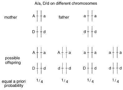
Suppose that the two loci are on different chromosomes. We |
then know the genotypes |
|
|
|||||||||||||||||
of the mother and the father unambiguously as shown in Figure 6.16. Independent segre- |
|
|
||||||||||||||||||
gation of alleles on different chromosomes leads to four possible genotypes for the off- |
|
|||||||||||||||||||
spring of these parents. A priori the probability of occurrence of each of these phenotypes |
1 |
|||||||||||||||||||
should |
be equal, so each |
should |
occur |
with |
an expected frequency of |
. Thus |
the a |
priori |
||||||||||||
4 |
||||||||||||||||||||
probability that the family in question should have both children with the same particular |
||||||||||||||||||||
|
||||||||||||||||||||
phenotype, AaDd is |
|
1 |
. We1 need to1 |
|
compare this probability, calculated from the |
|
||||||||||||||
|
|
|
|
|
4 |
|
4 |
16 |
|
|
|
|
|
|
|
|
|
|
|
|
hypothesis that the loci are unlinked, with the probability of seeing the same result if the |
|
|||||||||||||||||||
loci are linked. |
|
|
|
|
|
|
|
|
|
|
|
|
|
|
|
|
|
|||
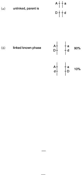
If the two loci are linked, they are on the same chromosome. In this case the genome of |
|
|||||||||||||||||||
the homozygous father can be described unambiguously, but there |
are |
two possible |
phases |
|
|
|||||||||||||||
for the mother. These are shown in Figure 6.17 |
|
|
|
|
|
a . Unless we have some a priori knowledge |
||||||||||||||
about the mother’s genotype, we must assume a priori that these two |
possible |
phases are |
1 |
|||||||||||||||||
equally probable. Thus there is a |
|
chance that the 1mother is cis and |
|
that she is trans. Since |
||||||||||||||||
|
|
|
|
|
|
|
|
|
|
2 |
|
|
|
|
|
|
|
|
2 |
|
we are not allowing for the possibility of recombination, if the mother is trans, the probability |
|
|||||||||||||||||||
that she would have an AaDd daughter is zero, since both the A and D alleles have to come |
|
|
||||||||||||||||||
from the mother in the family shown in Figure 6.15, and this |
would be impossible in the |
|
||||||||||||||||||
trans configuration where the A and D alleles are on different homologs. |
|
|
|
|
|
|
|
|||||||||||||
If the mother is cis for the two loci, there are two possible genotypes for any offspring. |
|
|||||||||||||||||||
These are shown in Figure 6.17 |
|
|
|
|
b . In the |
absence of any intervening factors, the a priori |
||||||||||||||
probability |
of |
observing |
these |
genotypes |
should |
be equal. Thus |
the |
chance |
of |
seeing |
a |
1 |
||||||||
child |
with |
the |
genotype |
AaDd under |
these |
circumstances is |
|
. The |
chance |
of |
a |
family |
||||||||
|
2 |
|||||||||||||||||||
with two children both of whom are AaDd will be |
|
|
|
. However, since1 |
we have1 |
no |
1 |
|||||||||||||
|
|
|
|
|
|
|
|
|
|
|
|
|
|
|
2 |
2 |
|
4 |
||
a priori knowledge about the phase of the mother, we must average the chances of seeing |
|
|
||||||||||||||||||
the expected offspring across both possible phases. The overall odds of the observed fam- |
|
|||||||||||||||||||
ily inheritance pattern is then |
|
|
|
1 |
|
1 |
1 |
|
1 |
|
|
|
|
|
||||||
|
|
|
2 |
(0) if |
(the)two loci are linked. |
|
|
|
||||||||||||
|
|
|
|
|
|
|
|
|
2 |
4 |
|
8 |
|
|
|
|
|
|||
Figure 6.16 Genotypes of the parents and expected offspring if the two loci and unlinked, and there is no recombination.

182 GENETIC ANALYSIS
Figure 6.17 |
Inheritance patterns with linkage, but no recombination. |
(a) |
Possible maternal geno- |
||
types |
if the two loci |
are linked. |
(b) Possible offspring if the mother |
is cis. For the example |
consid- |
ered, |
other offspring genotypes will be seen only if the loci are not linked. |
|
|
||
The odds ratio is a test of the likelihood that our hypothesis that linkage exists is correct. This is the ratio of the calculated probabilities with and without linkage:
|
|
P |
linked |
|
|
1 |
|
|
|
odds ratio |
|
|
|
8 |
|
|
2 |
||
P |
unlinked |
|
1 |
|
|
||||
|
|
|
|
|
|
|
|||
|
|
|
|
16 |
|
|
|
||
In human genetics we frequently know the phase of an individual because this |
is available |
|
|||||||
from data on other generations or other family members. In this case the odds ratio becomes |
|
||||||||
|
|
P |
linked |
|
|
1 |
|
|
|
odds ratio |
|
|
|
4 |
|
|
4 |
||
P |
unlinked |
|
1 |
|
|||||
|
|
|
|
|
|
|
|||
|
|
|
|
16 |
|
|
|
||
The greater power of linkage analysis with known phase is readily apparent.
With or without known phase, the single family shown in Figure 6.15 provides a small amount of statistical evidence in favor of linkage. To strengthen (or contradict) this evidence, we need to pool data from many such families. The overall odds ratio then becomes
P |
linked |
odds |
|
odds |
|
odds |
|
. . . |
|
P |
unlinked |
1 |
2 |
3 |
|||||
|
|
|
|
||||||
|
|
|
|
|
|
|
LINKAGE ANALYSIS WITH RECOMBINATION |
183 |
where the subscripts refer to different families under study. It is convenient mathematically to deal with a sum rather than a product of such data, and this is accomplished by taking the logarithm of both sides of the above equation. Since
|
|
|
|
log(A |
B C . . |
. ) log(A) |
log(B) |
log(C) . . . |
|||||
the result is |
|
|
|
|
|
|
|
|
|
|
|
||
|
|
|
LOD |
log |
|
P |
linked |
|
log(odds |
1 ) log(odds |
2) log(odds 3) . . . |
||
|
|
|
P |
unlinked |
|||||||||
|
|
|
|
|
|
|
|
|
|
||||
This is called a |
|
LOD |
(rhymes with cod) |
score. |
The LOD score is calculated from the data |
||||||||
seen with a particular family or set of families. Some feeling for the number of individu- |
|||||||||||||
als |
that |
must be |
examined for a LOD score to be statistically significant can be captured |
||||||||||
by |
the |
expected |
LOD score calculated for a particular inheritance model, called an |
||||||||||
ELOD. However, the inheritance model we use has to include the possibility of recombi- |
|||||||||||||
nation to be realistic enough to represent actual data. |
|
|
|
|
|||||||||
LINKAGE |
ANALYSIS |
WITH |
RECOMBINATION |
|
|
|
|
|
|
|
|||
Consider |
a pair |
of markers at loci that appear to be |
linked by available |
data. There |
are |
||||||||
three possible cases to deal with
1.The markers are unlinked, but random segregation gives the appearance of linkage.
2.The markers are really linked.
3.The markers are linked, but recombination has disguised this linkage.
We will deal with two markers as in the previous case. Here, however, it simplifies
matters if one of these is a locus where |
D is an allele of a disease gene |
that we are trying |
||
to find. A is an allele at another locus, |
and we are interested in testing |
the hypothesis |
that |
|
in a particular family A and D are linked. The chance that a recombination event occurs |
||||
between the two loci in each meiosis is an unknown variable |
|
. We need to calculate the |
||
odds in favor of linkage, for data from a particular family, as a function of |
. Actual |
|||
LOD( ) calculations are complex. To illustrate the considerations that go into such cal- |
||||
culations, we will calculate the expected contribution of a single individual observed to |
||||
inherit the disease allele D to the overall LOD score. This contribution is called the ex- |
||||
pected LOD or ELOD( |
). |
|
|
|
We will analyze the case where a parent is AaDd. Usually we are dealing with a rela- |
||||
tively rare disease, and the other parent does not have the D allele. We assume for sim- |
||||
plicity that the healthy parent |
also either has the a allele or some other allele that |
we can |
||
distinguish from A and a. We look only at offspring that are detected to carry the disease |
|
allele D. If the two loci are unlinked, the offspring inherit pairs of two different chromo- |
|
somes carrying A or a and D or d at random, as shown in Figure 6.18 |
a . We look only at |
offspring carrying D; thus there is a 0.5 probability that such an offspring will also inherit |
|
A. |
|
184 GENETIC ANALYSIS
Figure 6.18 Analysis of the inheritance of a disease allele D and a possible linked allele A. |
(a) |
Possible parental contributions to an offspring if no linkage occurs. |
(b) Possible parental contribu- |
tions to an offspring if the loci are linked but the recombination frequency between them is 0.1. |
|
We will consider the case where |
two |
loci |
are linked |
and |
the phase |
in |
the |
parent |
is |
known to be cis (Fig. 6.18 |
b ). What we want to calculate |
is |
the |
effect |
of observing one |
||||
child of this parent on the odds in |
favor |
of |
linkage of A |
and |
D. Suppose that |
|
is 0.1. |
||
Such a 10% chance of recombination corresponds to an average distance of 10 Mb in the genome. This is near the maximum distance across which linkage is visible in the analysis of only two loci at once. We can calculate the chance of two outcomes:
1.Probability that a child with D inherits AD from the parent is 0.9.
2.Probability that a child with D inherits aD from the parent is 0.1.
The contribution of case 1 to the expected LOD score is
log 00..95
which is the ratio of the odds of seeing A and D with linkage versus without linkage. The contribution of case 2 to the expected LOD score is
log 00..15
which is the ratio of the odds seeing aD with linkage to the odds of seeing aD without linkage.