

Berrar D. et al. - Practical Approach to Microarray Data Analysis
.pdf174 |
Chapter 9 |
instance of the Tikhonov regularization principle (Tikhonov and Arsenin, 1977).
Given a data set  the SVM algorithm takes this training set and finds a function
 The error of this function on the training set is called the empirical error, and we can measure it using Equation 9.12:
However, what we really care about is how accurate we will be given a new data sample, which is In general, we want to weight this error by the probability of drawing the sample
  and average this over all possible data samples. This weighted measure is called the expected or generalization error.
where p(x,y) is the distribution which the data is drawn from.
For algorithms that implement Tikhonov regularization, one can say with high probability (Bousquet and Elisseeff, 2002, Mukherjee et al., 2002):
where the function  decreases as
  decreases (or margin increases) and l increases. This tells us that if our error rate on the training set is low and the margin is large, then the error rate on average for a new sample will also be low. This is a theoretical motivation for using regularization algorithms such as SVMs. Note, that for the number of samples typically seen in
microarray expression problems, plugging in values of l and into |
will |
not yield numbers small enough to serve as practical error bars. |
|
2.2An Application of SVMs
One of the first cancer classification studies was discriminating acute myeloid leukemia (AML) from acute lymphoblastic leukemia (ALL) (Golub et al., 1999). In this problem, a total of 38 training samples belong to the two classes, 27 ALL cases vs. 11 AML cases. The accuracy of the trained classifier was assessed using 35 test samples. The expression levels of 7,129 genes and ESTs were given for each sample. A linear SVM trained on this data accurately classified 34 of 35 test samples (see Figure 9.6.)

9. Classifying Microarray Data Using Support Vector Machines |
175 |
From Figure 9.6 an intuitive argument can be formulated: the larger the absolute value of the signed distance,  the more confident we can be in
the classification. |
There exist approaches to convert the real-valued f(x) into |
confidence values |
(Mukherjee et al., 1999, Platt, 1999). Thus, |
we can classify samples that have a confidence value larger than a particular threshold, whereas the classification of samples with confidence values below this threshold will be rejected. We applied this methodology in (Mukherjee et al., 1999) to the above problem, with a positive threshold of
and a negative threshold of |
|
A simple rule of thumb value to use as threshold is |
Function |
values greater than this threshold are considered high confidence. This value is in general too large to use for rejections.
Polynomial or Gaussian kernels did not increase the accuracy of the classifier (Mukherjee et al., 1999). However, when “important” genes were removed, the polynomial classifier did improve performance. This suggests that correlation information between genes can be helpful. Therefore, we removed 10 to 1,000 of the most “informative” genes from the test and training sets according to the signal-to-noise (S2N) criterion (see Section 3.1). We then applied linear and polynomial SVMs on this data set and reported the error rates (Mukherjee et al., 1999). Although the differences are not statistically significant, it is suggestive that until the removal of 300 genes, the polynomial kernel improves the performance, which suggests that modeling correlations between genes helps in the classification task.
176 |
Chapter 9 |
3.GENE SELECTION
It is important to know which genes are most relevant to the binary classification task and select these genes for a variety of reasons: removing noisy or irrelevant genes might improve the performance of the classifier, a candidate list of important genes can be used to further understand the biology of the disease and design further experiments, and a clinical device recording on the order of tens of genes is much more economical and practical than one requiring thousands of genes.
The gene selection problem is an example of what is called feature selection in machine learning (see Chapter 6 of this volume). In the context of classification, feature selection methods fall into two categories filter methods and wrapper methods. Filter methods select features according to criteria that are independent of those criteria that the classifier optimizes. On the other hand, wrapper methods use the same or similar criteria as the classifier. We will discuss two feature selection approaches: signal-to-noise (S2N, also known as P-metric) (Golub et al., 1999, Slonim et al., 2000;), and recursive feature elimination (RFE) (Guyon et al., 2002). The first approach is a filter method, and the second approach is a wrapper method.
3.1Signal-to-Noise (S2N)
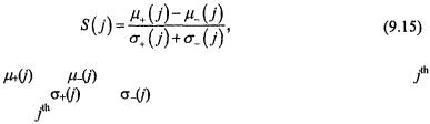
For each gene j, we compute the following statistic:
where |
and |
are the means of the classes +1 and –1 for the |
||
gene. Similarly, |
and |
are the standard deviations for the two |
||
classes for the |
|
gene. |
Genes that give the most positive values are most |
|
correlated with class +1, and genes that give the most negative values are most correlated with class –1. One selects the most positive m/2 genes and the most negative m/2 genes, and then uses this reduced dataset for classification. The question of estimating m is addressed in Section 3.3.
3.2Recursive Feature Elimination (RFE)
The method recursively removes features based upon the absolute magnitude of the hyperplane elements. We first outline the approach for linear SVMs. Given microarray data with n genes per sample, the SVM outputs the normal to the hyperplane, w, which is a vector with n components, each corresponding to the expression of a particular gene. Loosely speaking, assuming that the expression values of each gene have similar ranges, the

9. Classifying Microarray Data Using Support Vector Machines |
177 |
absolute magnitude of each element in w determines its importance in classifying a sample, since the following equation holds:
The idea behind RFE is to eliminate elements of w that have small magnitude, since they do not contribute much in the classification function. The SVM is trained with all genes; then we compute the following statistic for each gene:
Where  the value of the
  element of w. We then sort S from largest to smallest value and we remove the genes corresponding to the indices that fall in the bottom 10% of the sorted list S. The SVM is retrained on this smaller gene expression set, and the procedure is repeated until a desired number of genes, m, is obtained. When a nonlinear SVM is used, the idea is to remove those features that affect the margin the least, since maximizing the margin is the objective of the SVM (Papageorgiou et al., 1998). The nonlinear SVM has a solution of the following form:
Let M denote the margin. Then we obtain Equation 9.18:
So for each gene j, we compute to which extent the margin changes using the following statistic:
where  is the
 element of a vector of expression values x. We then sort S from the largest to the smallest value, and we remove the genes corresponding to the indices that fall in the bottom 10% of the sorted list S. The SVM is retrained and the procedure is repeated just as in the linear case.

178 |
Chapter 9 |
3.3How Many Genes To Use?
A basic question that arises for all feature selection algorithms is how many genes the classifier should use. One approach to answer this question is using hypothesis and permutation testing (Golub et al., 1999). The null hypothesis is that the S2N or RFE statistic for each gene computed on the training set comes from the same distribution as that for a random data set. A random data set is the training set with its labels randomly permuted.
In detail, the permutation test procedure for the S2N or RFE statistic is as follows:
(1)Generate the statistic for all genes using the actual class label and sort the genes accordingly.
(2)Generate 100 or more random permutations of the class labels. For each case of randomized class labels, generate the statistics for all genes and sort the genes accordingly.
(3)Build a histogram from the randomly permuted statistics using various numbers of genes. We call this number k. For each value of k, determine different percentiles (1%, 5%, 50% etc.) of the corresponding histogram.
(4)Compare the actual signal-to-noise scores with the different significance levels obtained for the histograms of permuted class labels for each value of k (see Figure 9.7 for an illustration).
4.ERROR RATES FOR MORPHOLOGY AND TREATMENT OUTCOME PREDICTION
We examined the error rate for SVMs and two other algorithms, Weighted Voting Average (WVA), and k-nearest neighbors (kNN) on seven binary

9. Classifying Microarray Data Using Support Vector Machines |
179 |
cancer classification problems. The problems are as follows: discriminating acute myeloid leukemia (AML) from acute lymphoblastic leukemia (ALL), and discriminating B-cells from T-cells for acute lymphoblastic leukemia (Golub et al., 1999), discriminating follicular (FSC) lymphoma from diffuse large cell lymphoma (DLCL) and discriminating high risk from low risk lymphoma patients (Shipp et al., 2001), discriminating glioblastomas (GL) from meduloblastomas (MD), and discriminating high risk from low risk patients with medulloblastoma (Pomeroy et al., 2002). See Table 9.1 for number of samples in each class for the data sets.
Error rates for all data sets except for AML vs. ALL were measured using leave-one-out cross validation4. For AML vs. ALL, the test/train split described in (Golub et al., 1999) was used. S2N was used for feature selection for WVA and kNN algorithms. The SVM used the radius-margin ratio as a gene selection methodology. The errors for both outcome prediction problems were much larger than those for the morphology prediction problems. The errors are reported in Table 9.2.
The number of genes used in each classification task for each algorithm was determined using cross-validation. In general, SVMs required more genes in the classification tasks.
4 See Chapter 7 of this volume for more details on leave-one-out cross-validation.

180 |
Chapter 9 |
5.MULTICLASS CLASSIFICATION
Ramaswamy et al. investigated whether the diagnosis of multiple adult malignancies could be achieved purely by molecular classification, using DNA microarray gene expression profiles (Ramaswamy et al., 2001). In total, 218 tumor samples, spanning 14 common tumor types, and 90 normal tissue samples were subjected to oligonucleotide microarray gene expression analysis. These tumor types/localizations are: breast (BR), prostate (PR), lung (LU), colorectal (CO), lymphoma (L), bladder (BL), melanoma (ME), uterus (UT), leukemia (LE), renal (RE), pancreas (PA), ovary (OV), mesothelioma (MS), and central nervous system (CNS). The expression levels of 16,063 genes and ESTs were used to train and evaluate the accuracy of a multiclass classifier based on the SVM algorithm. The overall classification accuracy was 78%, far exceeding the accuracy of random classification (9%). Table 9.3 shows the number of training and test samples per tumor class.

9. Classifying Microarray Data Using Support Vector Machines |
181 |
Multiple class prediction is intrinsically more difficult than binary prediction because the classification algorithm has to learn to construct a greater number of separation boundaries or relations. In binary classification, an algorithm can “carve out” the appropriate decision boundary for only one of the classes; the other class is simply the complement. In multiclass classification problems, each class has to be defined explicitly. A multiclass problem can be decomposed into a set of binary problems, and then combined to make a final multiclass prediction.
The basic idea behind combining binary classifiers is to decompose the multiclass problem into a set of easier and more accessible binary problems. The main advantage in this divide-and-conquer strategy is that any binary classification algorithm can be used. Besides choosing a decomposition scheme and a classifier for the binary decompositions, one also needs to devise a strategy for combining the binary classifiers and providing a final prediction. The problem of combining binary classifiers has been studied in the computer science literature (Hastie and Tibshirani, 1998, Allwein et al., 2000, Guruswami and Sahai, 1999) from a theoretical and empirical perspective. However, the literature is inconclusive, and the best method for combining binary classifiers for any particular problem is open.
Standard modern approaches for combining binary classifiers can be stated in terms of what is called output coding (Dietterich and Bakiri, 1991). The basic idea behind output coding is the following: given k classifiers trained on various partitions of the classes, a new example is mapped into an output vector. Each element in the output vector is the output from one of the k classifiers, and a codebook is then used to map from this vector to the class label (see Figure 9.7). For example, given three classes, the first classifier may be trained to discriminate classes 1 and 2 from 3, the second classifier is trained to discriminate classes 2 and 3 from 1, and the third classifier is trained to discriminate classes 1 and 3 from 2.
Two common examples of output coding are the one-versus-all (OVA) and all-pairs (AP) approaches. In the OVA approach, given k classes, k
independent classifiers are constructed where the |
classifier is trained to |
|
separate samples belonging to class i from all others. The codebook |
is a |
|
diagonal matrix, and the final prediction is based on the classifier |
that |
|
produces the strongest confidence: |
|
|
where is the signed confidence measure of the
  classifier (see Figure 9.8). In the all-pairs approach,
  classifiers are constructed, with each classifier trained to discriminate between a class pair i and j. This can be
5 The procedure arg maxf(x) simply selects the value or argument of x that maximizes f(x).

182 |
Chapter 9 |
thought of as a  matrix, where the
  entry corresponds to a classifier that discriminates between classes i and j. The codebook, in this case, is used to simply sum the entries of each row and select the row for which this sum is maximal:
where is the signed confidence measure for the
  classifier.
Intuitively, there is a tradeoff between the OVA and AP approaches. The discrimination surfaces that need to be learned in the all-pairs approach are, in general, more natural and, theoretically, should be more accurate. However, with fewer training examples, the empirical surface constructed may be less precise. The actual performance of each of these schemes, or others such as random codebooks, in combination with different classification algorithms is problem dependent. The OVA approach gave the best results on this dataset, and these results are reported in Table 9.4. The train/test split in the table is the same as that in (Ramaswamy et al., 2001). The error rate on the training set was measured using leave-one-out cross validation. A sample classification was considered high confidence if max and low confidence otherwise.

9. Classifying Microarray Data Using Support Vector Machines |
183 |
6.SOFTWARE SOURCES AND RULES OF THUMB
The SVM experiments described in this chapter were performed using a modified version of the SvmFu package, which can be downloaded from http://www.ai.mit.edu/projects/cbcl/). Another available SVM package is SVMTorch (http://www.idiap.ch/learning/SVMTorch.html). SvmFu has some advantages in that it has both multiclass and leave-one-out crossvalidation built in. SVMTorch is the only software of the above that does SVM regression as well as classification.
The following are some rules of thumb when using SVMs:
(1)Normalizing your data: in general it is a good idea to rescale your data such that all kernel values fall between –100 and 100; a simple
way to do this is by normalizing all entries of the microarray such that they fall between  and
and  where n is the number of expression values per sample;
(2)Choosing the regularization parameter C: given the above normalization, the regularization parameter usually does not have much effect, so set it somewhere between 1–100;
(3)Choosing the kernel: for microarray applications, a linear kernel is usually sufficient; you can use polynomial kernels if you want to examine correlations between genes, but it will in general not greatly improve the performance; if the linear kernel does not give good performance, it is worth trying the Gaussian kernel;
(4)Choosing the variance of the Gaussian kernel: set  such that the average distance between two training points
where l is the number of samples.
(5)Multiclass problems: for a multiclass problem, use the OVA and AP
decompositions; in general, more complicated coding systems do not help. When there are very few (5-10) training samples per class, OVA will in general give the best results.