Berrar D. et al. - Practical Approach to Microarray Data Analysis

average’ of M? One of the most popular methods is Lowess (Locally Weighted Regression) also referred to as Loess, which is a generic statistical technique for smoothing of data (Cleveland and Devlin, 1988; Hastie et al., 2001) and has been applied to microarray data by Dudoit et al. (2002) and Yang et al. (2002). Typically, Lowess fits a separate straight line through the data at every value of A. The slope, and intercept, for a particular value of interest, say, are determined predominantly by those data points with A values close to This is done using a window (or kernel) function, whose width is set so that only a fixed percentage f of the total data points are used in determining the slope and intercept at A popular choice of window function is the tri-cube function,

which we have used for the yeast data set. Typically the span f is set somewhere between 20% and 40% of the total data. The larger f, the more data is used to determine the straight line passing through If f is set too large, e.g., f close to 100%, the ‘local average’ produced by Lowess will be something close to a single straight line through all the data and consequently not follow the local variation or curvature of the M-A plot. If f is too small Lowess will follow the local variation of the M-A plot too closely and the ‘local average’ produced may be too wildly varying and affected by outliers in the M-A plot. For the example in Figure 4.3a we have

application of Lowess we refer the reader to Yang et al. (2002).

Lowess smoothing of the M-A plot is a very general technique and one can use the approach to correct for systematic variation introduced through sources other than dye bias, for example bias due to the particular print-tip with which the probe was printed onto the array, by making an M-A plot using those spots that have been printed using that particular print-tip. Such an approach has been investigated by Yang et al. (2002), to which we refer the reader for further details. After Lowess smoothing of M-A plots from several print-tips or several chips the user may still wish to bring the Lowess corrected ratios from the different data sets into a common scale. This can be done using the techniques outlined in the previous section, such as the total least-squares normalization method, or using the median absolute deviation (MAD) estimates of scale employed by Yang et al. (2002). For Lowess

corrected ratios from different print-tips, but a single hybridization, this would seem a very natural step.

When should one use Lowess smoothing of an M-A plot? Simply plotting the M-A values will give a good indication of whether a log intensity dependent correction of the ratio is required. This may be impractical when normalizing many chips and the user may wish to implement Lowess smoothing of M-A plots by default. The concern would then be the computational cost in doing this. In theory a locally weighted regression is performed at every value of A for which a corrected log-ratio is required, i.e. for every spot on the array. In theory this makes normalization using Lowess smoothing of an M-A plot considerably more computationally intensive than say mean or median centering of the log-ratio values. In practical terms, on modern desktop machines, there is not a dramatic difference in performance when normalizing a single chip. Lowess smoothing of the M-A plot shown in Figure 4.3a took 35 seconds on a 700MHZ Pentium III laptop using code written in Java. When performing normalization of many chips and/or print-tips, or normalization across multiple chips, speed maybe more of an issue. In such cases a locally weighted regression need not be done for every spot. Instead the observed range of A can be divided into a grid containing a finite number of points and a locally weighted regression performed at each of these grid points. Values of the smooth curve for values of A which do not lie at a grid point can be calculated by simple interpolation. Smoothing of the M-A plot in Figure 4.3a using a grid of 100 points took less than a second. If the same grid is used when normalizing many arrays a significant proportion of the calculation, the equivalent kernel, (Hastie et al., 2001) need only be done once, greatly improving the overall computational cost.

2.2.2.2 Paired-Slide Normalization

If we expect a significant number of genes to be differentially expressed, then correcting for dye-bias by smoothing of the M-A plot may not be appropriate, since we may not expect symmetric scatter of M values. In these circumstances elimination of dye-bias can be done with the use of paired slides, i.e. a dye-swap experiment in which two hybridizations are performed, with the labelling of sample and reference mRNA populations in one hybridization being the reverse of that in the other.

hybridization for the same probe. If the experiment were free from error,

However, from the M-A plots we have seen the bias would appear to depend

systematic intensity errors will approximately cancel out, even when we are considering genes that are differentially expressed, and so still represents a good estimate of the true log ratio at (Yang et al., 2001b). This is easily demonstrated using the yeast heat-shock dye-swap data. Figures 4.4a and 4.4b are M-A plots for the two individual

2.4Summary

The simple global linear transformations we started this section with can be used to correct for systematic errors that affect all spot intensities equally, e.g. differences in total mRNA between samples. However, the use of M-A plots has revealed significant log intensity dependant biases and therefore normalization using only a global transformation is likely to be inadequate. The use of Lowess to correct log intensity dependent bias is fast becoming a de facto standard for two-fluor spotted array data. We would recommend that users of spotted arrays should implement Lowess or another statistical smoothing technique. After correcting bias in several hybridizations these can be brought into a common scale using the global linear transformations discussed at the beginning of this section.

For non-spotted arrays, such as Affymetrix chips, correction of log intensity dependant bias can in principle be done by multi-dimensional nonlinear regression or non-linear regression to a reference chip.

So far we have not touched on the issue of spatial normalization. We have mentioned applying Lowess to spots just from the same print-tip, but this does not address the issue of bias that is dependent upon the actual physical location (planar coordinates) of the spot on the array. Such bias can arise due to uneven hybridization conditions across the array or contamination in a particular sector of the array. Plotting of log ratio values (from two-fluor spotted array data) against the 2D planar coordinates of the spots can reveal any biases. The local spatial behaviour of spot intensities, as a function of the spot coordinates, can be modelled using locally weighted regression in the 2D spot coordinates. Each regression calculation now involves two input variables – the spot coordinates – as opposed to one – the log intensity A – when performing standard Lowess normalization of an array. Consequently the computational cost is much higher, although for normalization of multiple arrays this can again be reduced if the regression calculations are always performed at the same spot locations – as might be appropriate when using arrays of similar design.

3.CONCLUSIONS

Normalization of microarray data is a complex issue and is unlikely to ever be cut and dried. Common sense and the user’s biological knowledge of the experiment can act as invaluable guides in the normalization process. As a minimum working practice we would recommend the following:

Always keep the raw data – normalization methods change. They can be improved or new ones invented. New sources of systematic error may be identified and algorithms constructed to eliminate them.

Maintain some sort of audit trail of what transformations (with what particular parameter settings) have been applied to your data.

Finally, as well as the research literature, one of the best places to keep abreast of developments in normalization techniques is by monitoring the efforts of the MGED normalization working group (http://www.mged.org).

ACKNOWLEDGEMENTS

We would like to thank Dr Abdulla Bashein for supplying the S. cerevisiae heat shock dye-swap data. We have also benefited from discussions with Prof. A. Brass, Dr. M. Rattray and Dr. Y, Fang. This work has been supported by the MRC (UK) and NERC (UK).

REFERENCES

Axon Instruments Inc. (2002). GenePix Software.

Available at http://www.axon.com/GN_Genomics.html#software.

Ball C.(2002). Systematic Bias in Microarray Data, presentation given at MGED IV, 13th16th Feb, Boston, USA. Available at http://www.dnachip.org/mged/normalization.html.

Chen Y., Dougherty E.R., Bittner ML. (1997). Ratio-based decisions and the quantitative analysis of cDNA microarray images. J. Biomed. Optics 2: 364-374.

Cleveland W.S., Devlin S.J. (1988). Locally weighted regression: an approach to regression analysis by local fitting, J. Am. Stat. Assoc. 83: 596-610.

Delbruck S., Ernst J.F. (1993). Morphogenesis-independent regulation of actin transcript levels in the pathogenic yeast Candida albicans. Mol Microbiol 10: 859-866.

Dudoit S., Yang Y.H., Callow M.J., Speed T.P. (2002). Statistical methods for identifying genes with differential expression in replicated cDNA microarray experiments, Statistica Sinica 12: 111-139. See also Technical Report #578. Available at http://stat-www.berkeley.edu/users/sandrine/publications.html.

Gasch A.P., Spellman P.T., Kao C.M., Carmel-Harel O., Eisen M.B., Storz G.,. Botstein D, Brown P.O. (2000). Genomic expression programs in the response of yeast cells to environmental changes. Mol Biol Cell 11: 4241-4257.

Goldsworthy S.M., Goldsworthy T.L., Sprankle C.S., Butterworth B.E, (1993). Variation in expression of genes used for normalization of Northern blots after induction of cell proliferation. Cell Prolif 26: 511-518.

Golub G.H., Van Loan C. (1979). Total Least Squares. In Smoothing Techniques for Curve Estimation, pp. 69-76. Springer-Verlag, Heidelberg.

Golub T.R., Slonim D.K., Tamayo P., Huard C., Gaasenbeek M., Mesirov J.P., Coller H., Loh M.L., Downing J.R., Caligiuri M.A., Bloomfield C.D., Lander E.S, (1999). Molecular classification of cancer: class discovery and class prediction by gene expression monitoring. Science 286: 531-537.

Hastie T., Tibishirani R., Friedman J. (2001). The Elements of Statistical Learning: Data Mining, Inference and Prediction. Springer, New York.

Heller R.A., Schena M., Chai A., Shalon D., Bedilion T., Gilmore J., Woolley D.E., Davis R.W. (1997). Discovery and analysis of inflammatory disease-related genes using cDNA microarrays. Proc Natl Acad Sci USA 94: 2150-2155.

Hill A.A., Brown E.L., Whitley M.Z., Tucker-Kellogg G., Hunter C.P., Slonim D.K. (2001). Evaluation of normalization procedures for oligonucleotide array data based on spiked cRNA controls. Genome Biol 2: RESEARCH0055.0051-0055.0013.

Huber P.J. (1981). Robust Statistics. Wiley, New York.

Huber W., Von Heydebreck A., Sultmann H., Poustka A., Vingron M. (2002). Variance stabilization applied to microarray data calibration and to the quantification of differential expression. Bioinformatics l(l):l-9.

Kerr M.K., Martin M., Churchill G.A. (2000). Analysis of variance for gene expression microarray data. J Comput Biol 7: 819-837.

Quackenbush J. (2001). Computational analysis of microarray data. Nat Rev Genet 2: 418427.

Rattray, M., N. Morrison, D.C. Hoyle, and A. Brass. 2001. DNA microarray normalization, PCA and a related latent variable model.: Technical Report. Available from http://www.cs.man.ac.uk/~magnus/magnus.html.

Schadt E.E., Li C., Ellis B., Wong W.H. (2001). Feature Extraction and Normalization Algorithms for High-Density Oligonucleotide Gene Expression Array Data. Journal of Cellular Biochemistry 37: 120-125.

Sherlock, G. 2001. Analysis of large-scale gene expression data. Brief Bioinform 2: 350-362.

Yang Y.H., Buckley M.J., Speed T.P. (2001a). Analysis of cDNA microarray images. Brief Bioinform 2: 341-349.

Yang Y.H., Dudoit S., Luu P., Lin D.M., Peng V., Ngai J., Speed T.P. (2002). Normalization for cDNA microarray data: a robust composite method addressing single and multiple slide systematic variation. Nucleic Acids Research 30: e15.

Yang Y.H., Dudoit S., Luu P., Speed T.P. (2001b). Normalization for cDNA microarray data. In Microarrays: Optical technologies and informatics. (eds. Bittner M.L., Chen Y., Dorsel A.N., and Dougherty E.R.), pp. See also Technical Report available at http://www.stat.berkeley.edu/users/terry/zarray/Html/papersindex.html. SPIE, Society for Optical Engineering, San Jose, CA.

Chapter 5

SINGULAR VALUE DECOMPOSITION AND PRINCIPAL COMPONENT ANALYSIS

Michael E. Wall1,2, Andreas Rechtsteiner1,3, Luis M. Rocha1

1 Computer and Computational Sciences Division, 2Bioscience Division, Los Alamos National Laboratory, Mail Stop B256, Los Alamos, New Mexico, 87545 USA,

e-mail: {mewall, rocha}@lanl.gov

3Systems Science Ph.D. Program, Portland State University, Post Office Box 751, Portland, Oregon 97207 USA,

e-mail: andreas@sysc.pdx.edu

1.INTRODUCTION

One of the challenges of bioinformatics is to develop effective ways to analyze global gene expression data. A rigorous approach to gene expression analysis must involve an up-front characterization of the structure of the data. Singular value decomposition (SVD) and principal component analysis (PCA) can be valuable tools in obtaining such a characterization. SVD and PCA are common techniques for analysis of multivariate data. A single microarray1 experiment can generate measurements for tens of thousands of genes. Present experiments typically consist of less than ten assays, but can consist of hundreds (Hughes et al., 2000). Gene expression data are currently rather noisy, and SVD can detect and extract small signals from noisy data.

The goal of this chapter is to provide precise explanations of the use of SVD and PCA for gene expression analysis, illustrating methods using simple examples. We describe SVD methods for visualization of gene expression data, representation of the data using a smaller number of variables, and detection of patterns in noisy gene expression data. In addition, we describe the mathematical relation between SVD analysis and Principal Component Analysis (PCA) when PCA is calculated using the

1 For simplicity, we use the term microarray to refer to all varieties of global gene expression technologies.

92 Chapter 5

covariance matrix, enabling our descriptions to apply equally well to either method. Our aims are 1) to provide descriptions and examples of the application of SVD methods and interpretation of their results; 2) to establish a foundation for understanding previous applications of SVD to gene expression analysis; and 3) to provide interpretations and references to related work that may inspire new advances.

In Section 1, the SVD is defined, with associations to other methods described. In Section 2, we discuss applications of SVD to gene expression analysis, including specific methods for SVD-based visualization of gene expression data, and use of SVD in detection of weak expression patterns. Our discussion in Section 3 gives some general advice on the use of SVD analysis on gene expression data, and includes references to specific published SVD-based methods for gene expression analysis. Finally, in Section 4, we provide information on some available resources and further reading.

1.1Mathematical definition of the SVD2

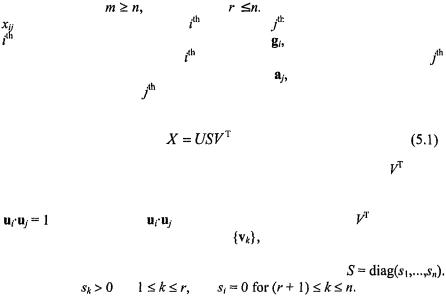
Let X denote an m × n matrix of real-valued data and rank3 r, where without

an n × n matrix. The columns of U are called the left singular vectors, and form an orthonormal basis for the assay expression profiles, so that

for the gene transcriptional responses. The elements of S are only nonzero on

2 Complete understanding of the material in this chapter requires a basic understanding of linear algebra. We find mathematical definitions to be the only antidote to the many confusions that can arise in discussion of SVD and PCA.

3 The rank of a matrix is the number of linearly independent rows or columns.

By convention, the ordering of the singular vectors is determined by high-to- low sorting of singular values, with the highest singular value in the upper left index of the S matrix. Note that for a square, symmetric matrix X, singular value decomposition is equivalent to diagonalization, or solution of the eigenvalue problem for X.

One important result of the SVD of X is that

is the closest rank-l matrix to X. The term “closest” means that minimizes the sum of the squares of the difference of the elements of X and This result can be used in image processing for compression and noise reduction, a very common application of SVD. By setting the small singular values to zero, we can obtain matrix approximations whose rank equals the number of remaining singular values. Each term is called a principal image. Very good approximations can often be obtained using only a small number of terms (Richards, 1993). SVD is applied in similar ways to signal processing problems (Deprettere, 1988) and information retrieval (Berry et al., 1995).

Choices for the remaining n - r singular vectors in V or U may be calculated using the Gram-Schmidt orthogonalization process or some other extension method. In practice there are several methods for calculating the SVD that are of higher accuracy and speed. Section 4 lists some references on the mathematics and computation of SVD.

Relation to principal component analysis. There is a direct relation between PCA and SVD in the case where principal components are calculated from the covariance matrix4. If one conditions the data matrix X