Berrar D. et al. - Practical Approach to Microarray Data Analysis

Our preference for PCA is based on the following arguments:

1.To allow for a biological interpretation of the ANN results, it is important that the connection between genes and ANN inputs can be easily reconstructed. Linear projections, e.g., PCA, fulfills this demand, in contrast to e.g., multi-dimensional scaling (Khan et al., 1998).

2. ANN analyses should involve cross-validation, described in Section 3.3. This implies that the ANN is trained several times, on different subsets of data, giving different parameter settings. An unsupervised dimensional reduction, e.g,. PCA, can use all available samples without introducing any bias. The result of this reduction can then be reused for every new training set. In contrast, a supervised reduction scheme can only rely on training samples to avoid bias, and must be redone as the training set changes.

3.In general, the N - 1 components containing all information are still too many for good ANN analyses. The ranking of principal components according to the variance gives information about inputs for which the separation of data points is robust against random fluctuations. Thus, PCA gives a hint on how to reduce the dimensionality further, without losing essential information.

4.The ANN inputs may need to be carefully selected, using a supervised evaluation of the components. The more correlated different input candidates are, the more difficult it is to select an optimal set. As principal components have no linear correlations, the PCA facilitates an efficient supervised selection of ANN inputs.

In Figure 11.2, the 63 SRBCT training samples, projected onto the first three principal components, are shown. Along component one there is a clear separation, poorly related to the four classes. This separation distinguishes tissue samples from cell-lines. This illustrates that the major principal components do not need to be the most relevant for the classification of interest. Thus, it can be useful to select ANN inputs using a supervised method. In doing so, we are helped by point 4 above. Since a central idea in the ANN approach is not to presume linear solutions, it is reasonable to use ANNs also for supervised input ranking.

A simple method is to train a network using quite many inputs (maybe even all). This network will most likely be heavily overfitted and is of little interest for blind testing, but can be used to investigate how the network performance on the training set is affected as one input is excluded. Doing so for each input gives information for input selection. In the SRBCT example, there was no need to do a supervised input selection, as the classification was successful using the 10 first principal components.

3CLASSIFICATION USING ANNS

3.1ANN Architecture

The simplest ANN-model is called a perceptron. It consists of an input layer and a single output (Figure 11.3). Associated with each input is a weight that decides how important that input is for the output. An input pattern can be fed into the perceptron and the responding output can be computed. The perceptron is trained by minimizing the error of this output. The perceptron is a linear classifier since the weights define a hyperplane that divides the input space into two parts.

In our example, we have four classes and a single perceptron does not suffice. Instead we use a system of four parallel perceptrons. Each perceptron is trained to separate one class from the rest, and as a classification the class with the largest output is chosen. It is recommended to first try a linear network. However, for more complicated problems a linear hyperplane is not good enough as a separator. Instead it is advantageous to have a nonlinear surface separating the classes. This can be achieved by using a multi-layer perceptron, in which several perceptrons are connected in a series (Figure 11.3).

Besides having an input and output layer, one also has one (or several) hidden layer(s) in between. The nodes in the hidden layer are computed from the inputs

where denotes the input and denotes the weights between the input and hidden layers.

The hidden nodes are used as input for the output (y) in the same manner

where denotes the weights between the hidden and output layers,

is the logistic sigmoid activation function, and

is the “tanh” activation function. A way to view this is that the input space is mapped into a hidden space, where a linear separation is done as for the linear perceptron. This mapping is not fixed, but is also included in the training. This means that the number of parameters, i.e. the number of weights, is much larger. When not having a lot of training samples this might cause overfitting. How many parameters one should use varies from problem to problem, but one should avoid using more than the number of training samples. The ANN is probabilistic in the sense that the output may easily be interpreted as a probability. In other words, we are modelling the probability that, given a certain information (the inputs), a sample belongs to a certain class (Hampshire and Pearlmutter, 1990).

3.2Training the ANN

Training, or calibrating, the network means finding the weights that give us the smallest possible classification error. There are several ways of measuring the error. A frequently used measure and the one we used in our example is the mean squared error (MSE)

where N is the number of training samples and and are the output and target for sample k and output node l, respectively. Since the outputs in classification are restricted (see Equations 11.2 and 11.3), the MSE is relatively insensitive to outliers, which typically results in a robust training

and a good performance on a validation set. Additionally, the MSE is computationally inexpensive to use in the training.

There is a countless number of training algorithms. In each algorithm there are a few training parameters that must be tuned by the user in order to get good and efficient training. Here, we will briefly describe the parameters in the gradient descent algorithm used in our example.

Given a number of input patterns and corresponding targets, the classification error can be computed. The error will depend on the weights and in the training we are looking for its minimum. The idea of the gradient descent can be illustrated by a man wandering around in the Alps, looking for the lowest situated valley. In every step he walks in the steepest direction and hopefully he will end up in the lowest valley. Below, we describe four parameters: epochs, step size, momentum coefficient and weight decay, and how they can be tuned.

The number of steps, epochs, is set by the user. It can be tuned using a plot of how the classification error change during the calibration (see Figure 11.4).

Using too few epochs, the minimum is not reached, yielding a training plot in which the error is not flattening out but still decreasing in the end.

Using too many epochs is time consuming, since the network does not change once a minimum is reached.

The step size is normally proportional to the steepness, and the proportionality constant is given by the user. How large the step size should be depends on the typical scale of the error landscape. A too large step size results in a coarse-grained algorithm that never finds a minimum. A fluctuating classification error indicates a too large step size. Using a too small step is time consuming.

3.3Cross-Validation and Tuning of ANNs

In the case of array data, where the number of samples typically is much smaller than the number of measured genes, there is a large risk of overfitting. That is, among the many genes, we may always find those that perfectly classify the samples, but have poor predictive ability on additional samples. Here, we describe how a supervised learning process can be carefully monitored using a cross-validation scheme to avoid overfitting. Of note, overfitting is not specific to ANN classifiers but is a potential problem with all supervised methods.

To obtain a classifier with good predictive power, it is often fruitful to take the variability of the training samples into account. One appealing way to do this is to construct a set of classifiers, each trained on a different subset of samples, and use them in a committee such that predictions for test samples are given by the average output of the classifiers. Thus, another advantage with using a cross-validation scheme is that it results in a set of ANNs that can be used as a committee for predictions on independent test samples in a robust way. In a cross-validation scheme there is a competition between having large training sets, needed for constructing good committee members, and obtaining different training sets, to increase the spread of predictions of the committee members. The latter results in a decrease in the committee error (Krogh and Vedelsby, 1995).

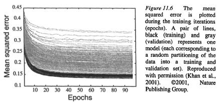
In general, 3-fold cross-validation is appropriate and it is the choice in the SRBCT example. In 3-fold cross-validation, the samples are randomly split into three groups. Two groups are used to train an ANN, and the third group is used for validation. This is repeated three times using each of the three groups for validation such that every sample is in a validation set once. To obtain a large committee, the random separation into a training and a validation set can be redone many times so that a set of ANNs are calibrated. The calibration of each ANN is then monitored by plotting both the classification error of the training samples and the validation samples as a function of training epochs (see Figure 11.6). A decrease in the training and the validation error with increasing epochs demonstrates the ability of the ANN to classify the experiments.

There are no general values for the learning parameters of ANNs, instead they can be optimized by trial and error using a cross-validation scheme. Overfitting results in an increase of the error for the validation samples at the point where the models begin to learn features in the training set that are not present in the validation set. In our example, there was no sign of overfitting (Figure 11.6).

Overfitting can for example be avoided by early stopping, which means that one sets the maximal number of training iterations to be less than where overfitting begins or by tuning the weight decay. In addition, by monitoring the cross-validation performance one can also optimize the architecture of the ANN, for example the number of inputs to use. When tuning ANNs in this way, it is important to choose a cross-validation scheme that does not give a too small number of samples left in each validation set.

Even though cross-validation can be used to assess the quality of supervised classifiers, it is always important to evaluate the prediction performance using an independent test set that has not been used when the inputs or the parameters of the classifier were optimized. The importance of independent test sets should be appreciated for all supervised methods.

3.4Random Permutation Tests

It is often stated that “black boxes” such as ANNs can learn to classify anything. Though this is not the case, it is instructive to evaluate if the classification results are significant. This can be accomplished using random permutation tests (Pesarin, 2001). In microarray analysis, random permutation tests have mostly been used to investigate the significance of genes with expression patterns that discriminate between disease categories of interest (Golub et al., 1999, Bittner et al., 2000). In our example, we randomly permute the target values for the samples and ANNs are trained to classify these randomly labeled samples. This random permutation of target values is performed many times to generate a distribution of the number of correctly classified samples that could be expected under the hypothesis of

random gene expression. This distribution is shown for the 63 SRBCT samples using 3-fold cross-validation to classify the samples in Figure 11.7.

The classification of the diagnostic categories of interest resulted in all 63 samples being correctly classified in the validation, whereas a random classification typically resulted in only 20 correctly classified samples. This illustrates the significance of the classification results for the diagnostic categories of the SRBCT samples.

3.5Finding the Important Genes

A common way to estimate the importance of an input to an ANN is to exclude it and see how much the mean squared error increases. This is a possible way to rank principal components, but the approach is ill suited for gene ranking. The large number of genes, many of which are correlated, implies that any individual gene can be omitted without any noticeable change of the ANN performance.

Instead, we may rank genes according to how much the ANN output is affected by a variation in the expression level of a gene, keeping all other gene expression levels and all ANN weights fixed. Since the ANN output is a continuous function of the inputs (cf. Section 3.1), this measure of the gene’s importance is simply the partial derivative of the output, with respect to the gene input. To get the derivative, it is important that the dimensional reduction is mathematically simple, so the gene’s influence on the ANN inputs can be easily calculated.

For well classified samples, the output is insensitive to all its inputs, as it stays close to 0 or 1 also for significant changes in the output function

argument. Not to reduce the influence of well classified samples on the gene ranking, one may instead consider as sensitivity measure the derivative, with respect to the gene input, of the output function argument.

There are problems where neither single input exclusion, nor sensitivity measures as above, identifies the importance of an input (Sarle, 1998). Therefore, the gene list obtained with the sensitivity measure should be checked for consistency, by redoing the analysis using only a few top-ranked genes. If the performance is equally good as before or better, the sensitivity measure has identified important genes. If the performance is worse, the sensitivity measure may be misleading, but it could also be that too few top genes are selected, giving too little information to the ANN.

In Figure 11.8, the ANN performance of the SRBCT classification, as a function of included top genes, is shown. The good result when selecting the top 96 genes shows that these genes indeed are relevant for the problem. One can also see that selecting only the six top genes excludes too much information. The performance measure in this example is the average number of validation sample misclassifications of an ANN. One can also consider less restrictive measures, like the number of misclassifications by the combined ANN committee. If so, it may be that less than 96 top genes can be selected without any noticeable reduction in the performance. When more than 96 genes were selected the average performance of the committee members went down. This increase in the number of misclassifications is likely due to overfitting introduced by noise from genes with lower rank. However, the combined ANN committee still classified all the samples correctly when more than 96 genes were used.

Once genes are ranked, it is possible to further study gene expression differences between classes. For example, one can check how many top genes can be removed without significantly reducing the performance.