

Berrar D. et al. - Practical Approach to Microarray Data Analysis
.pdf284 |
Chapter 16 |
with the smallest number of parameters.4 The classical k-means clustering algorithm has been shown to be closely related to this model (Celeux and Govaert, 1992). However, there are circumstances in which this model may not be appropriate. For example, if some groups of genes are much more tightly co-regulated than others, a model in which the spherical components are allowed to have different volumes may be more appropriate. The unequal volume spherical model (see Figure 16.2a),  allows the spherical components to have different volumes by allowing a different
  for each component k. We have also observed considerable correlation between experiments in time-series experiments, coupled with unequal variances. An elliptical model may better fit the data in these cases, for example, the unconstrained model (see Figure 16.2b) allows all of
 and
and  to vary between components. The unconstrained model has the advantage that it is the most general model, but has the disadvantage that the maximum number of parameters need to be estimated, requiring relatively more data points in each component. There is a range of elliptical models with other constraints, and hence requiring fewer parameters.
6.2Algorithm Outline
Assuming the number of clusters, G, is fixed, the model parameters are estimated by the expectation maximization (EM) algorithm. In the EM algorithm, the expectation (E) steps and maximization (M) steps alternate. In the E-step, the probability of each observation belonging to each cluster is estimated conditionally on the current parameter estimates. In the M-step, the model parameters are estimated given the current group membership probabilities. When the EM algorithm converges, each observation is assigned to the group with the maximum conditional probability. The EM algorithm can be initialized with model-based hierarchical clustering (Dasgupta and Raftery, 1998), (Fraley and Raftery, 1998), in which a maximum-likelihood pair of clusters is chosen for merging in each step.
6.3Model Selection
Each combination of a different specification of the covariance matrices and a different number of clusters corresponds to a separate probability model. Hence, the probabilistic framework of model-based clustering allows the issues of choosing the best clustering algorithm and the correct number of clusters to be reduced simultaneously to a model selection problem. This is important because there is a trade-off between probability model, and number of clusters. For example, if one uses a complex model, a small
4Only the parameter  needs to be estimated to specify the covariance matrix for the equal model spherical model.
16. Clustering or Automatic Class Discovery: non-hierarchical, non- |
285 |
SOM |
|
number of clusters may suffice, whereas if one uses a simple model, one may need a larger number of clusters to fit the data adequately.
Let D be the observed data, and  be a model with parameter
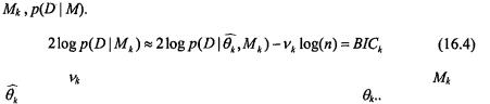
  The Bayesian Information Criterion (BIC) (Schwarz, 1978) is an approximation to the probability that data D is observed given that the underlying model is
where |
is the number of parameters to be estimated in model |
,and |
|
is the |
maximum likelihood estimate for parameter |
Intuitively, |
the |
first term in Equation 16.4, which is the maximized mixture likelihood for the model, rewards a model that fits the data well, and the second term discourages overfitting by penalizing models with more free parameters. A large BIC score indicates strong evidence for the corresponding model. Hence, the BIC score can be used to compare different models.
6.4Implementation
Typically, different models of the model-based clustering algorithm are applied to a data set over a range of numbers of clusters. The BIC scores for the clustering results are computed for each of the models. The model and the number of clusters with the maximum BIC score are usually chosen for the data. These model-based clustering and model selection algorithms (including various spherical and elliptical models) are implemented in MCLUST (Fraley and Raftery, 1998). MCLUST is written in Fortran with interfaces to Splus and R. It is publicly available at http://www.stat.washington.edu/fraley/mclust.
7.A CASE STUDY
We applied some of the methods described in this chapter to the yeast cell cycle data (Cho et al., 1998), which showed the fluctuation of expression levels of approximately 6,000 genes over two cell cycles (17 time points). We used a subset of this data, which consists of 384 genes whose expression levels peak at different time points corresponding to the five phases of cell cycle (Cho et al., 1998). We expect clustering results to approximate this five-class partition. Hence, the five phases of cell cycle form the external criterion of this data set.
Before any clustering algorithm is applied, the data is pre-processed by standardization, i.e. the expression vectors are standardized to have mean 0 and standard deviation 1 (by subtracting the mean of each row in the data,
286 Chapter 16
and then dividing by the standard deviation of the row). Data pre-processing techniques are discussed in detail in Chapter 2.
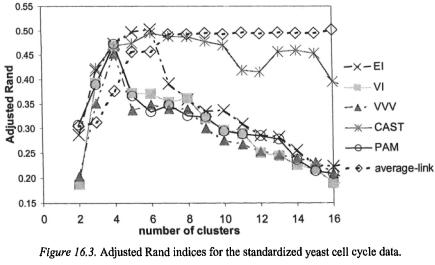
We applied CAST, PAM, hierarchical average-link and the model-based approach to the standardized yeast cell cycle data to obtain 2 to 16 clusters. The clustering results are evaluated by comparing to the external criterion of the 5 phases of cell cycle, and the adjusted Rand indices are computed. The results are illustrated in Figure 16.3. A high-adjusted Rand index means high agreement to the 5-phase external criterion. The results from three different models from the model-based approach are shown in Figure 16.3: the equal volume spherical model (denoted by EI), the unequal volume spherical model (denoted by VI), and the unconstrained model (denoted by VVV). The equal volume spherical model (EI) and CAST achieved the highest adjusted Rand indices at 5 clusters. Figure 16.4 shows a silhouette plot of the 5 clusters produced using PAM.

16. Clustering or Automatic Class Discovery: non-hierarchical, non- |
287 |
SOM |
|
Three of the five clusters show higher silhouette values than the other two, and hence, they are relatively more pronounced clusters. In each cluster, there are a few genes with very low silhouette values, and they represent outliers in the clusters.
REFERENCES
Anderberg, M.R. (1973). Cluster analysis for applications. Academic Press.
Baneld, J.D, and Raftery, A.E. (1993). Model-based Gaussian and non-Gaussian clustering. Biometrics, 49:803-821.
Ben-Dor, A., Shamir, R., and Yakhini, Z. (1999). Clustering gene expression patterns. Journal of Computational Biology, 6:281-297.
Ben-Dor, A, and Yakhini, Z. (1999). Clustering gene expression patterns. In RECOMB99: Proceedings of the Third Annual International Conference on Computational Molecular Biology, pages 33-42, Lyon, France.
Celeux, G. and Govaert, G. (1992). A classification EM algorithm for clustering and two stochastic versions. Computational Statistics and Data Analysis, 14:315-332.
Celeux, G. and Govaert, G. (1993). Comparison of the mixture and the classification maximum likelihood in cluster analysis. Journal of Statistical Computation and Simulation, 47:127-146.
Cho, R.J., Campbell, M.J., Winzeler, E.A., Steinmetz, L., Conway, A., Wodicka, L., Wolfsberg, T.G., Gabrielian, A. E., Landsman, D., Lockhart, D. J., and Davis, R. W. (1998). A genome-wide transcriptional analysis of the mitotic cell cycle. Molecular Cell, 2:65-73.
Dasgupta, A. and Raftery, A.E. (1998). Detecting features in spatial point processes with clutter via model-based clustering. Journal of the American Statistical Association, 93:294-302.
288 |
Chapter 16 |
Everitt, B. (1994). A handbook of statistical analyses using S-plus. Chap man and Hall, London.
Everitt, B.S. (1993). Clustering Analysis. John Wiley and Sons.
Fraley, C. and Raftery, A.E. (1998). How many clusters? Which clustering method? - Answers via model-based cluster analysis. The Computer Journal, 41:578-588.
Hartigan, J.A. (1975). Clustering Algorithms. John Wiley and Sons.
Hubert, L. and Arabie, P. (1985). Comparing partitions. Journal of Classification, 2:193-218.
Ihaka, R. and Gentleman, R. (1996). R: A language for data analysis and graphics. Journal of Computational and Graphical Statistics, 5(3):299-314.
Jain, A.K. and Dubes, R.C. (1988). Algorithms for Clustering Data. Prentice Hall, Englewood Cliffs, NJ.
Kaufman, L. and Rousseeuw, P.J. (1990), Finding Groups in Data: An Introduction to Cluster Analysts. John Wiley & Sons, New York.
Lander, E.S. et al. (2001). Initial sequencing and analysis of the human genome. Nature, 409(6822):860-921, International Human Genome Sequencing Consortium.
MacQueen, J. (1965). Some methods for classification and analysis of multivariate observations. In Proceedings of the 5th Berkeley Symposium on Mathematical Statistics and Probability, pages 281-297. McLachlan, G. J. and Basford, K. E. (1988). Mixture models: inference and applications to clustering. Marcel Dekker New York.
McLachlan, G.J. and Peel, D. (2000). Finite Mixture Models. New York: Wiley.
Rousseeuw, P. J. (1987). Silhouettes: a graphical aid to the interpretation and validation of cluster analysis. Journal of Computational and Applied Mathematics, 20:53-65.
Schwarz, G. (1978). Estimating the dimension of a model. Annals of Statistics, 6:461-464.
Selim, S.Z. and Ismail, M.A. (1984). K-means type algorithms: a generalized convergence theorem and characterization of local optimality. IEEE Transactions on Pattern Analysis and Machine Intelligence, PAMI-6(l):81-86.
Shamir, R. and Sharan, R. (2001). Algorithmic approaches to clustering gene expression data. In Current Topics in Computational Biology. MIT Press.
Tavazoie, S., Huges, J.D., Campbell, M.J., Cho, R.J., and Church, G.M. (1999). Systematic determination of genetic network architecture. Nature Genetics, 22:281-285.
Yeung, K.Y., Fraley, C., Murua, A., Raftery, A.E., and Ruzzo, W.L. (2001a). Model-based clustering and data transformations for gene expression data. Bioinformatics, 17:977-987.
Yeung, K.Y., Haynor, D.R., and Ruzzo, W.L. (2001b). Validating clustering for gene expression data. Bioinformatics, 17(4):309-318.
Yeung, K.Y. and Ruzzo, W.L. (2001). Principal component analysis for clustering gene expression data. Bioinformatics, 17:763-774.
Chapter 17
CORRELATION AND ASSOCIATION ANALYSIS
Simon M. Lin and Kimberly F. Johnson
Duke Bioinformatics Shared Resource, Box 3958, Duke University Medical Center, Durham, NC 27710,USA,
email: {Lin00025, Johns001}@mc.duke.edu
1.INTRODUCTION
Establishing an association between variables is always of interest in the life sciences. For example, is increased blood pressure associated with the expression level of the angiotensin gene? Does the PKA gene down-regulate the Raf1 gene?
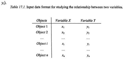
To answer these questions, we usually have a collection of objects (samples) and the measurements on two or more attributes (variables) of each object. Table 17.1 illustrates a collection of n pairs of observations 
In this chapter, we first define types of variables, the nature of which determines the appropriate type of analysis. Next we discuss how to statistically measure the strength between two variables and test their significance. Then we introduce machine learning algorithms to find
290 |
Chapter 17 |
association rules. Finally, after discussing the association vs. causality inference, we conclude with a discussion of microarray applications.
2.TYPES OF VARIABLES
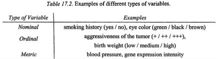
Different statistical procedures are developed for different types of variables. Here we define three types of variables. Nominal variables are orderless non-numerical categories, such as sex and marital status. Ordinal variables are ordered categories; sometimes they are also called rank variables. Different from nominal and ordinal variables, metric variables have numerical values that can be mathematically added or multiplied. Examples of different types of variables are in Table 17.2.
Sometimes it is convenient to convert the metric variables into ordinal variables. For example, rather than using the exact expression values of each gene, we discretize them into high, medium, and low values (Berrar et al., 2002). Although this conversion will lose some information from the original data, it makes the computation efficient and tractable, (Chang et al., 2002) or allows the use of algorithms for ordinal data (see Section 3.4; Chang et al., 2002).
3.MEASUREMENT AND TEST OF CORRELATION
In many situations it is often of interest to measure the degree of association between two attributes (variables) when we have a collection of objects (samples). Sample correlation coefficients provide such a numerical measurement. For example, Pearson’s product-moment correlation coefficient ranges from –1 to +1. The magnitude of this correlation coefficient indicates the strength of the linear relationship, while its sign indicates the direction. More specifically, –1 indicates perfect negative linear correlation; 0 indicates no correlation; and +1 indicates perfect positive linear correlation. According to the type of the variables, there are different formulas for calculating correlation coefficients. In the following sections, we will first discuss the most basic Pearson’s product moment correlation
17. Correlation and Association Analysis |
291 |
coefficient for a metric variable; then, rank-based correlation coefficients including Spearman’s rho and Kendall’s tau; and finally, Pearson’s contingency coefficient for nominal variables. Conceptually, there is a difference between the sample statistics vs. the true population parameters (Sheskin, 2000); for example, the sample correlation coefficient r vs. the population correlation coefficient  In the following discussion we focus on the summary statistics of the samples.
3.1Pearson’s Product-Moment Correlation Coefficient
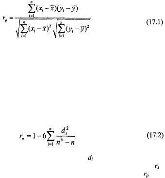
For metric variables, the Pearson’s product-moment correlation coefficient
(or Pearson’s rho) is calculated according to the following formula:
where  and
and  are the average of variable x and y, respectively. This formula measures the strength of a linear relationship between variable x and y. Since
  is the most commonly used correlation coefficient, most of the time it is referred to simply as r.
3.2Spearman’s Rank-Order Correlation Coefficient
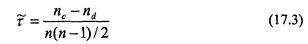
For ordinal variables, Spearman’s rank-order correlation coefficient (or, Spearman’s rho), is given by
where n is the total number of objects, and |
is the difference between |
||
the variable pair of rankings associated with the |
ith object. Actually, |
is |
|
simplified from Pearson’s product-moment correlation coefficient |
when |
||
the variable values are substituted with ranks. |
|
|
|
Spearman’s rho measures the degree of monotonic relationship between two variables. A relationship between two variables x and y is monotonic if, as x increases, y increases (monotonic increasing) or as x decreases, y decreases (monotonic decreasing).
292 |
Chapter 17 |
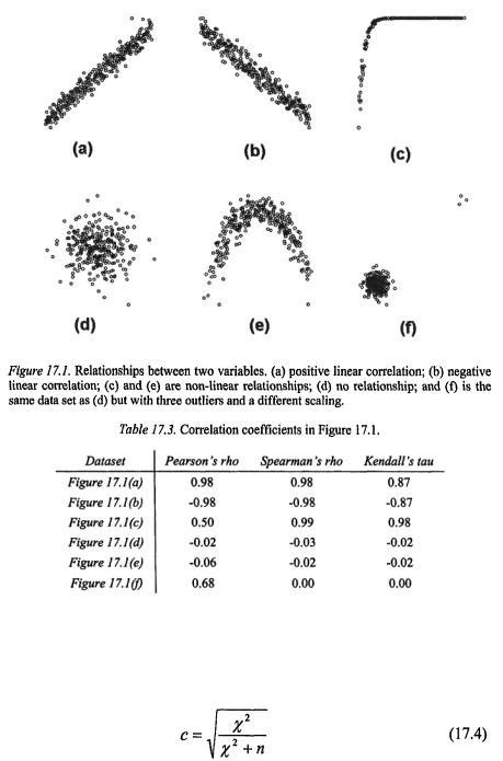
3.3Kendall’s Tau
As an alternative to Spearman’s rho, Kendall’s tau measures the proportional concordant pairs minus the proportional discordant pairs in samples, A pair of observations  and
and  is called concordant when the product
  is positive; and called discordant when the product is negative. Kendall’s tau is defined as
where is the number of concordant pairs of ranks,
  is the number of discordant pairs of ranks, and n(n – l)/2 is the total number of possible pairs of ranks.
3.4Comparison of Different Correlation Coefficients
Before we discuss the correlation coefficient for nominal variables, we first compare different correlation coefficients for ordinal and metric variables, since metric variables have the option of either using Pearson’s productmoment correlation, or being converted to rank order first, and then treated as ordinal variables.
Pearson’s rho measures the strength of a linear relationship (Figure 17.1a and Figure 17.1b), whereas Spearman’s rho and Kendall’s tau measure any monotonic relationship between two variables (Figure 17.1a, b, c and Table 17.2). If the relationship between the two variables is non-monotonic, all three correlation coefficients fail to detect the existence of a relationship (Figure 17.1e).
Both Spearman’s rho and Kendell’s tau are rank-based non-parametric measures of association between variable X and Y. Although they use different logic for computing the correlation coefficient, they seldom lead to markedly different conclusions (Siegel & Castellan, 1988).
The rank-based correlation coefficients are more robust against outliers. In Figure 17.1f, the data set is the same as in Figure 17.1d, except three outliers. As shown in Table 17.3, Spearman’s rho and Kendall’s tau are more robust against these outliers, whereas Pearson’s rho is not.
17. Correlation and Association Analysis |
293 |
3.5Pearson’s Contingency Coefficient
Pearson’s contingency coefficient (c) is a measurement of association for nominal data when they are laid out in a contingency table format. c is defined as: