


4
Empirical and Analytical
Correlations of Droplet
Properties
Atomization, or generally speaking droplet generation, is an extremely complex process that cannot yet be precisely predicted theoretically. The lack of general theoretical treatment of droplet processes has led to the development of numerous empirical correlations for droplet properties as a function of process parameters and material properties. In this chapter, empirical and analytical correlations for the prediction of droplet properties, such as droplet size distribution and droplet deformation characteristics will be summarized from experimental observations and theoretical analyses in available literature.
4.1.0CONCEPT AND DEFINITIONS OF DROPLET SIZE DISTRIBUTION
Droplet generation is typically a random process. Droplet sizes are usually characterized by a wide spectrum. In many
238
Empirical and Analytical Correlations 239
applications, mean droplet size and size distribution are the important factors to be controlled closely to achieve the desired rates of heat and mass transfer, or to meet specific application requirements because various dynamics and transport phenomena in droplet processes strongly depend on droplet size.
In most spray combustion systems, for example, droplet size frequency and spatial distribution govern fundamental flame characteristics such as heat transfer, flame length and stability, and emissions. A decrease in mean droplet size results in a higher heat release rate, easier lightup, a wider burning range, and a lower exhaust concentration of pollutant emissions. A uniform distribution of droplet sizes in spray may not always be desirable, since very small droplets are needed to provide high initial fuel evaporation rates for rapid ignition.
In spray deposition processes for near-net shape manufacturing, a small mean droplet size and narrow size distribution may lead to a refined microstructure and improved mechanical properties of as-sprayed preforms. However, in some other applications, such as agricultural aviation for crop spray,[88] small droplets of chemicals may not be desired under certain meteorological conditions because they can drift too far downwind due to their low settling velocities which might damage nearby crops, or present hazards to susceptible animals and human beings. On the other hand, excessively large droplets settle directly on the ground, resulting in nonuniform deposit of chemicals. Hence, both small and large droplets may cause inaccurate application of chemicals to the target area. Therefore, in such applications, the droplet size distribution needs to be controlled properly, and an atomization technique that can produce monodisperse sprays may be one of the solutions to eliminate the problems.
However, a monodisperse spray seldom exists in reality and is difficult to produce, although it can be defined mathematically as a spray consisting of droplets of the same size. Hence, a monodisperse spray usually refers to a spray in which droplets are very narrowly distributed. However, it is merely a relative term since a droplet size distribution that is sufficiently narrow in one application may be
240 Science and Engineering of Droplets
considered disperse in another. Thus, the choice of the exact criterion is sometimes arbitrary. In certain applications, a monodisperse spray is defined as a spray in which 95% of droplets are smaller than 1.2 times the average droplet size, and 5% of droplets are smaller than 0.8 times the average size.[88]
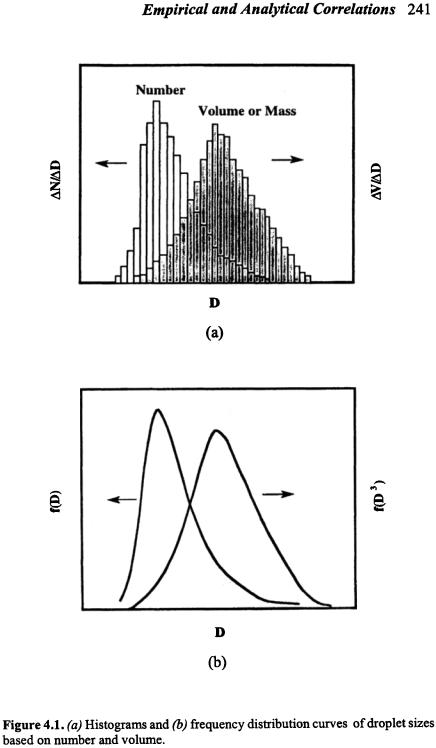
Droplet size distribution can be represented both graphically and mathematically. As a histogram of droplet size, both droplet number increment Ni / Di, and volume increment Vi / Di can be plotted vs. droplet size D (Fig. 4.1), where i is the size range considered, Ni is the number of droplets in size range i, Di is the middle diameter of size range i, and Ni and Vi are the number and volume increment within Di, respectively. The histogram based on volume is skewed to the right due to the weighting effect of larger droplets:
Eq. (1) |
Vi |
= N i |
|
π |
Di3 |
|
6 |
||||||
|
|
|
|
|||
As D is made smaller, a histogram becomes a frequency distribution curve (Fig. 4.1) that may be used to characterize droplet size distribution if samples are sufficiently large. In addition to the frequency plot, a cumulative distribution plot has also been used to represent droplet size distribution. In this graphical representation (Fig. 4.2), a percentage of the total number, total surface area, total volume, or total mass of droplets below a given size is plotted vs. droplet size. Therefore, it is essentially a plot of the integral of the frequency curve.
Mathematical representation of droplet size distribution has been developed to describe entire droplet size distribution based on limited samples of droplet size measurements. This can overcome some drawbacks associated with the graphical representation and make the comparison and correlation of experimental results easier. A number of mathematical functions and empirical equations[423]-[427] for droplet size distributions have been proposed on the basis of
Empirical and Analytical Correlations 243
distribution functions in order to find the best fit to a set of experimental data unless the precise mechanism of atomization in the droplet generation device has been understood and related to one or more distribution functions. For the selection of a suitable distribution function, the consistency with the physical phenomena involved and mathematical/computational simplicity/ease are some factors to be considered.
Many droplet size distributions in random droplet generation processes follow Gaussian, or normal distribution pattern. In the normal distribution, a number distribution functionf(D) may be used to determine the number of droplets of diameter D:
|
|
dN |
|
|
1 |
|
é |
1 |
|
|
2 ù |
||
|
|
|
|
|
|
||||||||
Eq. (2) |
f (D) = |
|
= |
|
|
|
expê- |
|
(D - D ) |
ú |
|||
dD |
|
|
|
2 |
|||||||||
2π sn |
|||||||||||||
|
|
|
|
ë |
2sn |
|
|
|
û |
||||
where sn is the standard deviation, a measure of the deviation of values of D from the mean value D¯, and sn2 is the variance. A plot of the distribution function is the so-called standard normal curve, the area under which from –¥ to +¥ equals 1. The integral of the standard normal distribution function is the cumulative standard number distribution function F(D):
|
|
|
|
|
|
|
|
|
|
|
|
|
|
2 |
|
|
|
|
|
|
Eq. (3) |
F(D) = |
|
1 |
|
D |
|
é |
1 æ D - |
D ö |
ù æ D - D ö |
||||||||||
|
|
|
|
|||||||||||||||||
|
|
|
|
|
|
ç |
|
|
|
÷ |
|
úd ç |
|
|
|
÷ |
||||
|
|
|
|
expê- |
|
|
|
|
|
|
|
|
||||||||
|
|
ò |
2 |
s |
|
|
|
s |
|
|
||||||||||
|
|
|
2π |
|
ê |
ç |
n |
÷ |
|
ú |
ç |
n |
÷ |
|||||||
|
|
|
|
|
−∞ |
ë |
|
è |
|
ø |
|
û |
è |
|
ø |
|||||
Plotting droplet size data on an arithmetic-probability graph paper will generate a straight line if the data follow normal distribution. Thus, the mean droplet diameter and standard deviation can be determined from such a plot.
Many droplet size distributions in natural droplet formation and liquid metal atomization processes conform to lognormal distribution:

244 |
Science and Engineering of Droplets |
|
|
|
|
|
||||||||
|
|
|
dN |
|
|
1 |
é |
1 |
|
|
|
2 |
ù |
|
|
|
|
|
|
|
|
|
|||||||
Eq. |
(4) |
f (D) = |
|
= |
|
|
|
expê- |
|
(lnD - lnD |
ng |
) |
ú |
|
dD |
|
|
|
2sg2 |
||||||||||
|
|
|
|
|
2π Dsg |
ê |
|
|
|
ú |
||||
|
|
|
|
|
|
|
|
ë |
|
|
|
|
|
û |
where D¯ng is the number geometric mean droplet diameter and sg is the geometric standard deviation. Plotting droplet size data on a log-probability graph paper will generate a straight line if the data follow log-normal distribution.
Log-normal distribution functions based on surface and volume, respectively, are:
|
f (D2 ) = |
|
1 |
é |
|
|
1 |
(lnD - ln |
|
|
)2 |
ù |
|||
Eq. (5) |
|
expê- |
D |
sg |
ú |
||||||||||
|
|
|
2sg2 |
||||||||||||
|
|
|
|
2π Dsg |
ê |
|
|
|
|
|
|
ú |
|||
|
|
|
|
|
|
ë |
|
|
|
|
|
|
|
|
û |
and |
|
|
|
|
|
|
|
|
|
|
|
|
|
|
|
Eq. (6) |
f (D3 ) = |
|
|
1 |
é |
- |
|
1 |
(ln D - ln |
|
|
|
)2 |
ù |
|
|
|
expê |
|
D |
|
ú |
|||||||||
|
|
|
|
|
|
||||||||||
|
|
|
|
2π Dsg |
ê |
|
|
2sg2 |
|
|
vg |
|
ú |
||
|
|
|
|
|
|
ë |
|
|
|
|
|
|
|
|
û |
where D¯sg and D¯vg are the geometric surface and volume mean droplet diameters, respectively. These diameters can be determined once the number geometric mean droplet diameter and the geometric standard deviation are known:
Eq. (7) |
ln |
|
|
= ln |
|
|
+ 2s2 |
|
|
D |
D |
ng |
|
||||||
|
|
sg |
|
|
|
g |
|
||
Eq. (8) |
ln |
|
|
= ln |
|
|
+ 3s 2 |
|
|
D |
D |
ng |
|
||||||
|
|
vg |
|
|
|
g |
|
||
Eq. (9) |
ln SMD = ln |
|
|
+ 2.5s2 |
|||||
D |
ng |
||||||||
|
|
|
|
|
|
|
|
g |
|

Empirical and Analytical Correlations 245
In many atomization processes of normal liquids, droplet size distributions fairly follow root-normal distribution pattern:[264]
|
|
dN |
|
|
1 |
|
é |
1 |
|
2 ù |
||
Eq. (10) |
f (D) = |
|
= |
|
|
|
expê- |
|
((D /MMD)1/2 |
-1) |
ú |
|
dD |
|
|
|
2 |
||||||||
2π ss |
||||||||||||
|
|
|
|
ë |
2ss |
|
|
û |
||||
where ss is the standard deviation. This distribution function generates satisfactory fitting to the data from atomization experiments with a large number of gas-turbine fuel nozzles of different types, over a range of fuel viscosities, and at a variety of operation conditions.[264] In this distribution, a straight line can be generated by plotting (D /MMD)0.5 vs. cumulative volume of droplets on a normal-probability scale. This distribution is simpler than the log-normal and Rosin-Rammler distributions.
Nukiyama, and Tanasawa[79] proposed a relatively simple function for adequate description of some actual droplet size distributions:
Eq. (11) |
f (D) = |
dN |
= aD p exp[− bD q ] |
|
|||
|
|
dD |
|
where a, b and p are constants and q is the dispersion coefficient which is a constant for a given nozzle design. The value of q usually varies from 1/6 to 2, and is determined by trial-and-error. A graphical method to determine a and b has been proposed by Mugele and Evans.[423] In the Nukiyama-Tanasawa distribution equation, p = 2, such that:
Eq. (12) |
f (D) = |
dN |
= aD 2 exp[− bD q ] |
|
|||
|
|
dD |
|
Rearranging this equation, it reduces to:
246 Science and Engineering of Droplets
|
æ |
1 |
|
dN ö |
= ln a - bD |
q |
||
Eq. (13) |
lnç |
|
|
|
|
÷ |
|
|
D |
2 |
|
|
|||||
|
è |
|
|
dD ø |
|
|
||
Plotting ln[1/D2(dN /dD)] vs. D q based on experimental data and an assumed value of q, a straight line may be generated if the assumed q value is correct. Thus, the values of a and b can be determined from the plot so that the entire droplet size distribution can be characterized with the function.
Rosin-Rammler distribution function[428] is perhaps the most widely used one at present:
Eq. (14) |
V = 1 - exp[- D / X ]q |
where V is the fraction of total volume of droplets smaller than D, and X and q are constants. The exponent q is a measure of the spread of droplet sizes. A larger value of q corresponds to a more uniform droplet size. For many droplet generation processes, q ranges from 1.5 to 4, and for rotary atomization processes, q may be as large as 7. For those atomization processes that generate uniform droplet sizes, q is infinite. A straight line can be generated by plotting ln(1 – V)-1 vs. droplet diameter on a normal-probability scale. The value of q can be then obtained as the slope of the line, and the value of X equals the value of D corresponding to 1 – V = exp(–1), i.e., V = 0.632. RosinRammler distribution function assumes an infinite range of droplet sizes and therefore allows data to be extrapolated down to the range of very small droplet sizes where measurements are most difficult and least accurate.
Mugele and Evans[423] proposed the upper-limit distribution function based on their analyses of various distribution functions and comparisons with experimental data. This distribution function is a modified form of the log-normal distribution function, and for droplet volume distribution it is expressed as:

Empirical and Analytical Correlations 247
|
dV |
é |
1 |
|
|
2 |
|
2 ù |
|
Eq. (15) |
|
= δ expê- |
|
|
|
δ |
|
y |
ú |
dy |
|
|
|
|
|||||
π |
|
||||||||
|
ë |
|
|
|
|
û |
|||
where y = ln [aD/(Dmax – D)], δ is a factor related to the standard deviation of droplet size, a is a dimensionless constant, and Dmax is
the maximum droplet diameter. The Sauter mean diameter is formulated as:
Eq. (16) |
SMD = |
Dmax |
|
1 + a exp(1/ 4δ 2 ) |
|||
|
|
The upper-limit distribution function assumes a finite minimum and maximum droplet size, corresponding to a y value of –¥ and +¥, respectively. The function is therefore more realistic. However, similarly to other distribution functions, it is difficult to integrate and requires the use of log-probability paper. In addition, it usually requires many trials to determine a most suitable value for a maximum droplet size.
Some other distribution functions have also been derived from analyses of experimental data,[429][430] or on the basis of probability theory.[431] Hiroyasu and Kadota[317] reported a more generalized form of droplet size distribution, i.e., χ -square distribution. It was shown that the χ -square distribution fits the available spray data very well. Moreover, the χ -square distribution has many advantages for the representation of droplet size distribution due to the fact that it is commonly used in statistical evaluations.
It has been indicated[323] that for some distributions it is possible to find, at least, an empirical correlation between the mean droplet size and the standard deviation. Gretzinger and Marshall[102] have proposed such empirical equations relating the mean droplet size and the standard deviation for water-air system. Thus, once the mean droplet size is determined from a mathematical model, an empirical correlation, and/or experimental data, the entire droplet size distribution can be then predicted quantitatively.
248 Science and Engineering of Droplets
In many applications, a mean droplet size is a factor of foremost concern. Mean droplet size can be taken as a measure of the quality of an atomization process. It is also convenient to use only mean droplet size in calculations involving discrete droplets such as multiphase flow and mass transfer processes. Various definitions of mean droplet size have been employed in different applications, as summarized in Table 4.1. The concept and notation of mean droplet diameter have been generalized and standardized by Mugele and Evans.[423] The arithmetic, surface, and volume mean droplet diameter (D10, D20, and D30) are some most common mean droplet diameters:
|
|
|
|
Dmax |
|
|
|
|
|
Eq. (17) |
D10 |
= |
òDmin D(dN / dD)dD |
|
|
|
|||
|
Dmax |
(dN / dD)dD |
|
|
|||||
|
|
|
|
òDmin |
|
|
|||
|
|
|
é |
òDDmax |
D 2 (dN / dD)dD ù1 / 2 |
||||
Eq. (18) |
D20 |
= |
ê |
min |
|
|
|
ú |
|
ê |
|
|
|
|
ú |
||||
Dmax |
(dN / dD)dD |
|
|||||||
|
|
|
ê |
òD |
|
ú |
|||
|
|
|
ë |
min |
|
|
û |
||
|
|
|
é |
òDDmax D3 (dN / dD)dDù1 / 3 |
|||||
Eq. (19) |
D30 |
= |
ê |
min |
|
|
|
ú |
|
ê |
|
|
|
ú |
|||||
Dmax |
(dN / dD)dD |
||||||||
|
|
|
ê |
òD |
|
ú |
|||
|
|
|
ë |
min |
|
|
û |
||
where Dmin is the minimum droplet diameter. The arithmetic mean droplet diameter is the linear average diameter of all droplets in a sample. The volume mean droplet diameter represents the diameter of a droplet whose volume, multiplied by the total number of droplets, equals the total volume of the sample. A general form of mean droplet diameter can be written as:[423]
Eq. (20)
or
Eq. (21)
Dab
Dab
Empirical and Analytical Correlations 249
|
é |
òDDmax |
D a (dN / dD)dD ù1/( a−b ) |
|
= |
ê |
min |
ú |
|
ê |
|
|
ú |
|
Dmax |
|
|||
|
ê |
òDmin |
Db (dN / dD)dD ú |
|
|
ë |
û |
||
é åN i Dia ù1 /(a−b)
= ê åN Db ú êë i i úû
where a and b may take any values according to the effect considered, as listed in Table 4.1. Among these, the Sauter mean diameter SMD is perhaps the most widely used one. It represents the diameter whose ratio of volume to surface area is the same as that of the entire droplet sample. Analyses[1] showed that for combustion applications only SMD can properly indicate the fineness of a spray, thus SMD is to be used to describe atomization quality.
To characterize a droplet size distribution, at least two parameters are typically necessary, i.e., a representative droplet diameter, (for example, mean droplet size) and a measure of droplet size range (for example, standard deviation or q). Many representative droplet diameters have been used in specifying distribution functions. The definitions of these diameters and the relevant relationships are summarized in Table 4.2. These relationships are derived on the basis of the Rosin-Rammler distribution function (Eq. 14), and the diameters are uniquely related to each other via the distribution parameter q in the Rosin-Rammler distribution function. Lefebvre[1] calculated the values of these diameters for q ranging
from 1.2 to 4.0. The calculated results showed that Dpeak is always larger than SMD, and SMD is between 80% and 84% of Dpeak for many droplet generation processes for which 2 £ q £ 2.8. Thus, SMD
always lies on the left-hand side of Dpeak . The ratio MMD/SMD is
250 Science and Engineering of Droplets
always greater than one, and it changes only very little for q ³ 3; D0.9 is more than double MMD for q £ 1.7, but it is only 50% higher than MMD for q = 3.
Table 4.1. Definitions of Mean Droplet Diameters and Their
Applications[423]
Quantity |
Common |
a |
b |
|
Definition |
Application |
|||
Name |
|
||||||||
|
|
|
|
|
|
|
|
|
|
D10 |
Arithmetic |
1 |
0 |
|
å N i Di |
Comparison |
|||
Mean |
|
å |
N i |
|
|||||
|
(Length) |
|
|
|
|
|
|||
|
|
|
|
|
|
|
|||
|
Surface Mean |
|
|
æ |
|
|
2 |
ö1 / 2 |
Surface Area |
D20 |
|
|
ç |
å N i Di |
÷ |
||||
(Surface Area) |
2 |
0 |
ç |
å N i |
÷ |
Controlling |
|||
|
è |
ø |
|||||||
|
|
|
|
|
|
|
|
|
|
D30 |
Volume Mean |
|
|
æ |
|
|
3 |
ö1 / 3 |
Volume |
3 |
0 |
ç |
å Ni Di |
÷ |
Controlling |
||||
|
(Volume) |
ç |
å N i |
÷ |
|||||
|
|
|
(Hydrology) |
||||||
|
|
|
è |
ø |
|||||
D21 |
Length Mean |
|
|
|
å |
N i Di2 |
|
||
(Surface |
2 |
1 |
|
|
|
|
Absorption |
||
|
|
å N i Di |
|||||||
|
Area-Length) |
|
|
|
|
||||
|
|
|
|
|
|
|
|
|
|
D31 |
Length Mean |
|
|
æ |
|
|
3 |
ö1 / 2 |
Evaporation, |
(Volume- |
3 |
1 |
ç |
å Ni Di |
÷ |
Molecular |
|||
|
ç |
å Ni Di |
÷ |
||||||
|
Length) |
|
|
Diffusion |
|||||
|
|
|
è |
ø |
|||||
D32 |
Sauter Mean |
|
|
|
å N i Di3 |
Mass |
|||
(SMD) |
3 |
2 |
|
å N i Di2 |
Transfer, |
||||
|
(Volume- |
|
|||||||
|
Surface) |
|
|
|
|
|
|
|
Reaction |
|
|
|
|
|
|
|
|
|
|
D43 |
Herdan Mean |
|
|
|
å N i Di4 |
Combustion, |
|||
(De Brouckere |
4 |
3 |
|
å N i Di3 |
|||||
|
or Herdan) |
|
Equilibrium |
||||||
|
(Weight) |
|
|
|
|
|
|
|
|
|
|
Empirical and Analytical Correlations |
251 |
||||||||||||||||||||||||||
Table 4.2. Definitions of Representative Droplet Diameters |
|
|
|
|
|||||||||||||||||||||||||
|
|
|
|
|
|
|
|
|
|
|
|
|
|
|
|
|
|
|
|
|
|
|
|
|
|
|
|
|
|
|
Symbol |
Definition |
Position in V- |
|
|
|
|
|
|
|
|
|
|
Relationship |
|
|
|
|
|||||||||||
|
D plot |
|
|
|
|
|
|
|
|
|
|
|
|
|
|
||||||||||||||
|
|
|
|
|
|
|
|
|
|
|
|
|
|
|
|
|
|
|
|
|
|
|
|
|
|
|
|
|
|
|
|
10% of total |
|
|
|
|
|
|
|
D0.1 |
|
|
|
|
|
|
|
|
|
|
1 / q |
|
|
|
|
||||
|
|
volume of droplets |
|
|
|
|
|
|
|
|
|
|
|
|
|
= |
(0.1054) |
|
|
|
|
||||||||
|
D0.1 |
|
|
|
|
|
|
|
|
X |
|
|
|
|
|
|
|||||||||||||
|
are of smaller |
V=10% |
|
|
|
|
|
|
|
|
|
|
|
|
|
|
|
|
|
|
|
|
|
|
|
||||
|
|
|
|
|
|
|
|
D0.1 |
|
|
|
|
|
|
|
|
|
|
|
||||||||||
|
|
diameters than this |
|
|
|
|
|
|
|
|
= (0.152)1/ q |
|
|
|
|
||||||||||||||
|
|
|
|
|
|
|
|
MMD |
|
|
|
|
|||||||||||||||||
|
|
value |
|
|
|
|
|
|
|
|
|
|
|
|
|
|
|
|
|||||||||||
|
|
Mass median |
|
|
|
|
|
|
|
MMD |
|
|
|
|
|
|
|
|
|
|
|
|
|||||||
|
|
diameter |
V=50% |
|
|
|
|
|
|
|
= (0.693)1 / q |
|
|
|
|
||||||||||||||
|
D0.5 |
|
|
|
|
|
|
|
|
|
|
|
|
|
|
||||||||||||||
|
50% of total |
Left-hand or |
|
|
|
|
|
|
|
|
X |
|
|
|
|
|
|
|
|
|
|
|
|
|
|
|
|||
|
(MMD) |
volume of droplets |
right-hand side |
|
|
|
MMD |
|
|
|
|
|
|
|
|
|
|
|
æ |
1 ö |
|
||||||||
|
|
|
|
|
|
|
|
|
|
|
|
|
|
|
|
|
|
||||||||||||
|
are of smaller |
of Dpeak for q > |
|
|
|
|
|
|
|
|
|
|
= (0.693)1/ q Gç1- |
|
÷ |
|
|||||||||||||
|
|
|
|
|
|
|
|
|
|
|
|
|
|||||||||||||||||
|
|
diameters than this |
or < 3.2584 |
|
|
|
SMD |
|
|
|
|
|
|
|
|
|
|
|
ç |
q |
÷ |
|
|||||||
|
|
|
|
|
|
|
|
|
|
|
|
|
|
|
|
è |
ø |
|
|||||||||||
|
|
value |
|
|
|
|
|
|
|
|
|
|
|
|
|
|
|
|
|
|
|
|
|
|
|
|
|
|
|
|
|
Characteristic |
|
|
|
|
|
|
|
|
|
|
|
|
|
|
|
|
|
|
|
|
|
|
|
|
|
|
|
|
|
diameter |
|
|
|
|
|
|
|
|
|
|
|
|
|
|
|
|
|
|
X |
|
|
|
|
|
|
|
|
|
D0.632 |
63.2% of total |
V=63.2% |
|
|
|
|
|
|
|
|
|
|
|
|
|
|
|
|
|
|
|
|
|
|
|
|
|
|
|
|
volume of droplets |
|
|
|
|
(X in Rosin-Rammler |
|
|
|
|||||||||||||||||||
|
|
are of smaller |
|
|
|
|
|
distribution function) |
|
|
|
||||||||||||||||||
|
|
diameters than this |
|
|
|
|
|
|
|
|
|
|
|
|
|
|
|
|
|
|
|
|
|
|
|
|
|
|
|
|
|
value |
|
|
|
|
|
|
|
|
|
|
|
|
|
|
|
|
|
|
|
|
|
|
|
|
|
|
|
|
|
90% of total |
|
|
|
|
|
|
|
D0.9 |
|
|
= (2.3025)1/ q |
|
|
|
|
||||||||||||
|
D0.9 |
|
|
|
|
|
|
|
|
X |
|
|
|
|
|
|
|
||||||||||||
|
volume of droplets |
V=90% |
|
|
|
|
|
|
|
|
|
|
|
|
|
|
|
|
|
|
|
|
|
|
|
||||
|
|
are of smaller |
|
|
|
|
|
|
|
D0.9 |
= (3.32)1/ q |
|
|
|
|
||||||||||||||
|
|
diameters than this |
|
|
|
|
|
|
|
|
|
|
|
|
|||||||||||||||
|
|
|
|
|
|
|
|
|
MMD |
|
|
|
|
||||||||||||||||
|
|
value |
|
|
|
|
|
|
|
|
|
|
|
|
|
|
|
|
|
||||||||||
|
|
|
|
|
|
|
|
|
|
|
|
|
|
|
|
|
|
|
|
|
|
|
|
|
|
|
|
|
|
|
|
Maximum diameter |
|
|
|
|
|
|
|
|
|
|
|
|
|
|
|
|
|
|
|
|
|
|
|
|
|
|
|
|
D0.999 |
99.9% of total |
|
|
|
|
|
|
|
D0.999 |
|
= (9.968)1 / q |
|
|
|
|
|||||||||||||
|
|
volume of droplets |
V=99.9% |
|
|
|
|
|
|
|
|
|
|
||||||||||||||||
|
|
|
|
|
|
MMD |
|
|
|
|
|||||||||||||||||||
|
|
are of smaller |
|
|
|
|
|
|
|
|
|
|
|
|
|
|
|
|
|||||||||||
|
|
diameters than this |
|
|
|
|
|
|
|
|
|
|
|
|
|
|
|
|
|
|
|
|
|
|
|
|
|
|
|
|
|
value |
|
|
|
|
|
|
|
|
|
|
|
|
|
|
|
|
|
|
|
|
|
|
|
|
|
|
|
|
|
|
|
|
|
|
|
|
|
|
D peak |
|
æ |
|
1 |
ö1/ q |
|
|
|
|
|||||||||
|
|
|
|
|
|
|
|
|
|
|
|
|
|
|
|
|
|
|
|
= |
ç1- |
|
|
÷ |
|
|
|
|
|
|
|
|
|
|
|
|
|
|
|
|
|
|
|
|
|
|
|
|
|
|
|
|
|
|
|
||||
|
|
Peak diameter |
|
|
|
|
|
|
|
|
|
|
X |
|
|
|
|
|
|
ç |
|
q |
÷ |
|
|
|
|
||
|
|
|
|
|
|
|
|
|
|
|
|
|
|
|
|
|
|
è |
|
ø |
|
|
|
|
|||||
|
Dpeak |
Value of D |
Peak point |
|
D |
peak |
|
|
|
æ |
|
|
|
|
|
|
1.4428 |
ö1/ q |
|
||||||||||
|
corresponding to |
corresponding |
|
|
|
|
= |
ç1.4428- |
÷ |
|
|
|
|||||||||||||||||
|
|
|
|
|
|
|
|
|
|
||||||||||||||||||||
|
|
peak of droplet size |
|
MMD |
|
ç |
|
|
|
|
|
|
|
q |
÷ |
|
|
|
|||||||||||
|
|
to d2v/dD2=0 |
|
|
è |
|
|
|
|
|
|
|
ø |
|
|
|
|||||||||||||
|
|
frequency |
|
|
|
D peak |
|
æ |
|
|
|
1 |
ö1/ q |
æ |
1 |
ö |
|
||||||||||||
|
|
distribution curve |
|
|
|
|
|
|
- |
|
|||||||||||||||||||
|
|
|
|
|
|
|
|
|
|
|
|
|
= ç1 |
|
÷ |
|
|
Gç1- |
|
|
÷ |
|
|||||||
|
|
|
|
|
|
|
SMD |
|
ç |
|
|
|
q |
÷ |
|
|
ç |
q |
|
÷ |
|
||||||||
|
|
|
|
|
|
|
|
è |
|
|
|
ø |
|
|
è |
ø |
|
||||||||||||
|
|
|
|
|
|
|
|
|
|
|
|
|
|
|
|
|
|
|
|
|
|
|
|
|
|
|
|
|
|
|
|
|
|
|
|
|
|
|
|
|
|
|
|
|
|
|
|
|
|
|
|
|
|
|
|
|
|
|
|
252 Science and Engineering of Droplets
Since the ratio of any two representative diameters is a unique function of q, Rosin-Rammler distribution function can be rewritten as:
Eq. (22)
or
Eq. (23)
é
V =1 - exp ê-
ê
ë
é
V =1 - expê-
ê
ë
æ |
D öq ù |
||
0.693ç |
|
÷ |
ú |
|
|||
è |
MMD ø |
ú |
|
|
|
|
û |
æ |
|
1 |
ö |
− q |
æ |
D ö |
q ù |
|
Gç1 |
- |
|
÷ |
|
ç |
|
÷ |
ú |
|
|
|
||||||
ç |
|
q |
÷ |
|
è SMD ø |
ú |
||
è |
|
ø |
|
|||||
|
|
|
|
|
|
|
|
û |
where Γ denotes the gamma function. Since these formulations clearly show both the fineness and the spread of droplet sizes in a spray, their applications are strongly recommended.[1] Based on these equations and those relationships in Table 4.2, representative diameters such as SMD, MMD, D0.1 and D0.9 can be determined once q is determined from experimental data.
It should be indicated that a probability density function has been derived on the basis of maximum entropy formalism for the prediction of droplet size distribution in a spray resulting from the breakup of a liquid sheet.[432] The physics of the breakup process is described by simple conservation constraints for mass, momentum, surface energy, and kinetic energy. The predicted, most probable distribution, i.e., maximum entropy distribution, agrees very well with corresponding empirical distributions, particularly the RosinRammler distribution. Although the maximum entropy distribution is considered as an ideal case, the approach used to derive it provides a framework for studying more complex distributions.
The ratio MMD/SMD is generally recognized as a good measure of droplet size range. In addition, various indices and factors have been defined to describe the spread of droplet sizes in a
spray, for example, droplet uniformity index ΣVi(MMD - Di)/MMD[433]
ι
and relative span factor (D0.9 – D0.1)/MMD, etc.