Enzymes (Second Edition)

130 KINETICS OF SINGLE-SUBSTRATE ENZYME REACTIONS

Figure 5.8 Lineweaver—Burk double-reciprocal plot for selected data from Table 5.1 within the range of [S] 0.25—5.0Km .

Thus if the reciprocal of initial velocity is plotted as a function of the reciprocal of [S], we would expect from Equation 5.34 to obtain a linear plot. For the same reasons described earlier for untransformed data, these plots work best when the substrate concentration covers the range of 0.25—5.0K . Within this range, good linearity is observed, as illustrated in Figure 5.8 for the data between [S] 3.91 and [S] 62.50 M in Table 5.1. A plot like that in Figure 5.8 is known as a Lineweaver—Burk plot.

The kinetic constants K and V can be determined from the slope and intercept values of the linear fit of the data in a Lineweaver—Burk plot. Since the x axis is reciprocal substrate concentration, the value of x 0 (i.e., 1/[S] 0) corresponds to [S] infinity. Hence, the extrapolated value of the y intercept corresponds to the reciprocal of V . The value of K can be determined from a Lineweaver—Burk plot in two ways. First we note from

We have noted several times that the preferred way to determine K and V values is from nonlinear fitting of untransformed data to the Michaelis— Menten equation. Figure 5.8 illustrates why we have stressed this point. In real experimental data, small errors in the measured values of v are amplified by the mathematical transformation of taking the reciprocal. The greatest percent error is likely to be associated with velocity values at low substrate concentration. Unfortunately, in the reciprocal plot, the lowest values of [S] correspond

to the highest values of 1/[S], and because of the details of linear regression, these data points are weighted more heavily in the analysis. Hence the experimental error is amplified and unevenly weighted in this analysis, resulting in poor estimates of the kinetic constants even when the experimental error is relatively small. To illustrate this, let us compare the estimates of V and K obtained for the data in Table 5.1 by various graphical methods; this is

summarized in Table 5.2. The true values of V and K for the hypothetical

data in Table 5.1 were 100 M/s and 12 M, respectively. The fitting of the untransformed data to the Michaelis—Menten equation provided estimates of 100.36 and 11.63 for the two kinetic constants, with deviations from the true values of only 0.36 and 3.08%, respectively. The linear fitting of the data in Figure 5.8, on the other hand, yields estimates of V and K of 91.84 and 9.17, with deviations from the true values of 8.16 and 23.58%, respectively. The errors are even greater when the double-reciprocal plots are used for the full data set in Table 5.1, as illustrated in Figure 5.9 and Table 5.2. Here the inclusion of the low substrate data values ( [S] 3.91 M) are very heavily weighted in the linear regression and further limit the precision of the kinetic constant estimates. The values of V and K derived from this fitting are 79.28 and 7.57, representing deviations from the true values of 20.72 and 36.92%, respectively.

The foregoing example, should convince the reader of the limitations of using linear transformations of the primary data for determining the values of the kinetic constants. Nevertheless, the Lineweaver—Burk plots are still commonly used by many researchers and, as we shall see in later chapters, are valuable tools for certain purposes. In these situations (described in detail in Chapters 8 and 11), we make the following recommendation. Rather than using linear regression to fit the reciprocal data in Lineweaver—Burk plots, one should determine the values of V and K by nonlinear regression analysis of the untransformed data fit to the Michaelis—Menten equation. These values are then inserted as constants into Equation 5.34 to create a line through the

132 KINETICS OF SINGLE-SUBSTRATE ENZYME REACTIONS

Figure 5.9 Lineweaver—Burk double-reciprocal plot for the full data set from Table 5.1. Note the strong influence of the data points at low [S] (high 1/[S] values) on the best fit line from linear regression.

reciprocal data on the Lineweaver—Burk plot. The line drawn by this method may not appear to fit the reciprocal data as well as a linear regression fit, but it will be a much more accurate reflection of the kinetic behavior of the enzyme. The use of this method will be more clear when it is applied in Chapters 8 and 11 to studies of enzyme inhibition and multisubstrate enzyme mechanisms, respectively.

If one is to ultimately present experimental data in the form of a doublereciprocal plot, it is desirable to chose substrate concentrations that will be evenly spaced along a reciprocal x axis (i.e., 1/[S]). This is easily accomplished experimentally as follows. One picks a maximum value of [S] ([S ]) to work with and makes a stock solution of substrate that will give this final concentration after dilution into the assay reaction mixture. Additional initial velocity measurements are then made by adding the same final volume to the enzyme reaction mixture from stock substrate solutions made by diluting the original stock solution by 1:2, 1:3, 1:4, 1:5, and so on. In this way, the data points will fall along the 1/[S] axis at intervals of 1, 2, 3, 4, 5, . . . , units.

For example, let us say that we have decided to work with a maximum substrate concentration of 60 M in our enzymatic reaction. If we prepare a 600 M stock solution of substrate for this data point, we might dilute it 1:10 into our assay reaction mixture to obtain the desired final substrate concentration. If, for example, our total reaction volume were 1.0 mL, we could start our reaction by mixing 100 L of substrate stock, with 900 L of the other components of our reaction system (enzyme, buffer, cofactors, etc.). Table 5.3 summarizes the additional stock solutions that would be needed to prepare final substrate concentrations evenly spaced along a 1/[S] axis.

Table 5.3 Setup for an experimental determination of enzyme kinetics using a Linewever--Burk plot

5.7 OTHER LINEAR TRANSFORMATIONS OF ENZYME KINETIC DATA

Despite the errors associated with this method, the Lineweaver—Burk doublereciprocal plot has become the most popular means of graphically representing enzyme kinetic data. There are, however, a variety of other linearizing transformations. Again, the use of these transformation methods is no longer necessary because most researchers have access to computer-based nonlinear curve-fitting methods, and the direct fitting of untransformed data by these methods is highly recommended. For the sake of historic persepective, however, we shall describe three other popular graphical methods for presenting enzyme kinetic data: Eadie—Hofstee, Hanes—Wolff, and Eisenthal—Cornish- Bowden direct plots. These linear transformation methods, which are here applied to enzyme kinetic data, are identical to the Wolff transformations described in Chapter 4 for receptor—ligand binding data.

134 KINETICS OF SINGLE-SUBSTRATE ENZYME REACTIONS

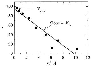
Figure 5.10 Eadie—Hofstee plot of enzyme kinetic data. Data taken from Table 5.1.

Hence, if we plot v as a function of v/[S], Equation 5.37 would predict a straight-line relationship with slope of K and y intercept of V . Such a plot, referred to as an Eadie—Hofstee plot, is illustrated in Figure 5.10.

5.7.2 Hanes‒Wolff Plots

If one multiplies both sides of the Lineweaver—Burk Equation (Equation 5.34) by [S], one obtains:

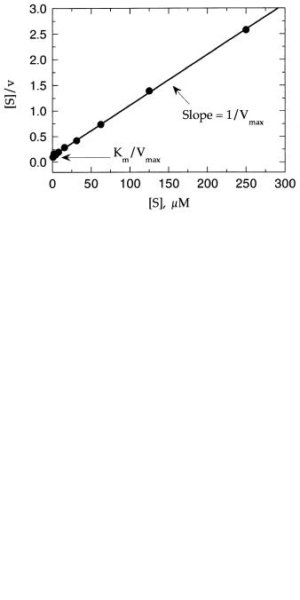
This treatment also leads to linear plots when [S]/v is plotted as a function of [S]. Figure 5.11 illustrates such a plot, which is known as a Hanes—Wolff plot. In this plot the slope is 1/V , the y intercept is K /V , and the x intercept is K .

5.7.3 Eisenthal‒Cornish-Bowden Direct Plots

In our final method, pairs of v, [S] data (as in Table 5.1) are plotted as follows: values of v along the y axis and the negative values of [S] along the x axis (Eisenthal and Cornish-Bowden, 1974). For each pair, one then draws a straight line connecting the points on the two axes and extrapolates these lines past their point of intersection (Figure 5.12). When a horizontal line is drawn from the point of intersection of these line to the y axis, the value at which this horizontal line crosses the y axis is equal to V . Similarly, when a vertical line is dropped from the point of intersection to the x axis, the value at which this

Figure 5.11 Hanes—Wolff plot of enzyme kinetic data. Data taken from Table 5.1.

vertical line crosses the x axis defines K . Plots like Figure 5.12, are referred to as Eisenthal—Cornish-Bowden direct plots and are considered to give the best estimates of K and V of any of the linear transformation methods. Hence they are highly recommended when it is desired to determine these kinetic parameters but nonlinear curve fitting to Equation 5.24 is not feasible.

Figure 5.12 Eisenthal—Cornish-Bowden direct plot of enzyme kinetic data. Selected data taken from Table 5.1.

5.9 DEVIATIONS FROM HYPERBOLIC KINETICS

In most cases enzyme kinetic measurements fit remarkably well to the Henri—Michaelis—Menten behavior discussed in this chapter. However, occasional deviations from the hyperbolic dependence of velocity on substrate concentration are seen. Such anomalies occur for several reasons. Some physical methods of measuring velocity, such as optical spectroscopies, can lead to experimental artifacts that have the appearance of deviations from the expected behavior, and we shall discuss these in detail in Chapter 7.

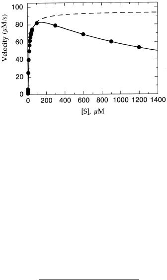
Nonhyperbolic behavior can also be caused by the presence of certain types of inhibitor as well. In the most often encountered case, substrate inhibition, a second molecule of substrate can bind to the ES complex to form an inactive ternary complex, SES. Because formation of the ES complex must precede formation of the inhibitory ternary complex, substrate inhibition is usually realized only at high substrate concentrations, and it is detected as a lower than expected value for the measured velocity at these high substrate concentrations. Figure 5.13 illustrates the type of behavior one might see for an enzyme that exhibits substrate inhibition. At low substrate concentrations, the kinetics follow simple Michaelis—Menten behavior. Above a critical substrate concentration, however, the data deviate significantly from the expected behavior. The binding of the second, inhibitory, molecule of substrate can be accounted for by the following equation:

or dividing the top and bottom of the right-hand side of Equation 5.43 by [S], we obtain:

where the term K in Equations 5.43 and 5.44 represents the dissociation constant for the inhibitory SES ternary complex. Inhibition effects at very high substrate concentrations also can be readily detected as nonlinearity in the Lineweaver—Burk plots of the data. Here one observes a sudden and dramatic curving up of the data near the y-axis intercept.

Another cause of nonhyperbolic kinetics is the presence of more than one enzyme acting on the same substrate (see also Chapter 4, Section 4.3.2.2). Many enzyme studies are performed with only partially purified enzymes, and many clinical diagnostic tests that rely on measuring enzyme activities are performed on crude samples (of blood, tissue homogenates, etc.). When the

138 KINETICS OF SINGLE-SUBSTRATE ENZYME REACTIONS

Figure 5.13 Michaelis—Menten plot for an enzyme reaction displaying substrate inhibition at high substrate concentrations: dashed line, best fit of the data at low substrate concentrations to Equation 5.24; solid line, fit of all the data to Equation 5.44. The constant Ki (Equation 5.44) will be described further in subsequent chapters.

substrate for the reaction is unique to the enzyme of interest, these crude samples can be used with good results. If, however, the sample contains more than one enzyme that can act on the substrate, deviations from the expected kinetic results occur. Suppose that our sample contains two enzymes; both can convert the substrate to product, but they display different kinetic constants. Suppose further that for one of the enzymes V V and K K , and for the second enzyme V V and K K . The velocity of the overall mixture then is given by:

Equation 5.46 is a polynomial expression, which yields behavior very different from the rectangular hyperbolic behavior we expect; this is illustrated in Figure 5.14.

One last example of deviation from hyperbolic kinetics is that of enzymes displaying cooperativity of substrate binding. In the derivation of Equation 5.24 we assumed that the active sites of the enzyme molecules behave independently of one another. As we saw in Chapter 3 and 4, sometimes proteins occur as multimeric assemblies of subunits. Some enzymes occur as

Figure 5.14 Effects of multiple enzymes acting on the same substrate. The dashed line represents the fit of the data to Equation 5.24 for a single enzyme, while the solid line represents the fit to Equation 5.46 for two enzymes acting on the same substrate with V1 120 M/s,

V2 75 M/s, K1 65 M, and K2 3 M.

homomultimers, each subunit containing a separate active site. It is possible that the binding of a substrate molecule at one of these active sites could influence the affinity of the other active sites in the multisubunit assembly (see Chapter 12 for more details). This effect is known as cooperativity. It is said to be positive when the binding of a substrate molecule to one active site increases the affinity for substrate of the other active sites. On the other hand, when the binding of substrate to one active site lowers the affinity of the other active sites for the substrate, the effect is called negative cooperativity. The number of potential substrate binding sites on the enzyme and the degree of cooperativity among them can be quantified by the Hill coefficient, h. The influence of cooperativity on the measured values of velocity can be easily taken into account by modifying Equation 5.24 as follows:

where K is related to K but also contains terms related to the effect of substrate occupancy at one site on the substrate affinity of other sites (see Chapter 12). Figure 5.15 illustrates how positive cooperativity can affect the Michaelis—Menten and Lineweaver—Burk plots of an enzyme reaction.

The velocity data for cooperative enzymes can be presented in a linear form by use of Equation 5.48: