192 DETERMINATION OF COMPLEX REACTION MECHANISMS

derive theoretical expressions for the dependence of the invariants on the concentrations. By checking the validity of these dependences for the experimental data we can test the validity of the assumed reaction mechanisms.

In conclusion, we have suggested that the linear response law and the response experiments can be applied to the study of dynamic behavior of complex chemical systems. We have shown that the response experiments make it possible to evaluate the susceptibility functions from transient as well as frequency response experiments. We have shown that the susceptibility functions bear important information about the mechanism and kinetics of complex chemical processes. We have suggested a method, based on the use of tensor invariants, which may be used for extracting information about reaction mechanism and kinetics from susceptibility measurements in time-invariant systems.

12.5Errors in Response Experiments

The experimental study of large chemical and biochemical systems involves simultaneous measurements of many variables, typically concentrations. Extracting kinetic information from such large amounts of data is not easy. One way of overcoming the complications due to nonlinear kinetics is to use small perturbations and use linearized kinetics for the analysis of experimental data. This is a popular approach in biochemistry and molecular biology (see for example [25]). Unfortunately, for small perturbations experimental errors are high, in the range of 20–30% or even higher, and thus the accuracy of the results obtained based on small perturbations is questionable. Compared to these methods, our approach has a big advantage; it is based on a linear response law which is not the result of a linearization procedure and is valid even for large perturbations and nonlinear kinetics.

In the following we analyze the influence of errors on our approach and its accuracy and compare the results with those obtained by using linearized kinetics. We consider a nonlinear kinetic example for which a detailed analytical study is possible. We compare that exact solution with the first-order response theory based on appropriate tracer measurements, and also compare it with the response of the linearized kinetic example. An important interest here is in the effects of error propagations in the analysis due to the application to measurements of poor precision.

We consider a simple test model which has the advantage that it can be studied analytically even for very large numbers of intermediates, which makes it suitable for the analysis of the interference between experimental errors with the errors due to linearization. This type of model, which is somewhat similar to Eigen’s hypercycle model [26], has recently been introduced in connection with a population genetic problem [12]. The model used here is essentially a space-independent, homogeneous version of the model from [12]. We assume that there are two types of chemical species in the system, stable chemicals, Av , v = 1, 2, . . . , and active intermediates Xu, u = 1, 2, . . . , and that there is a very large supply of stable species Av , v = 1, 2, . . . , and their concentrations av , v = 1, 2, . . . , are assumed to be constant and only the concentrations xu, u = 1, 2, . . . , of the active intermediates are variable. We consider that the active intermediates replicate, transform into each other, and disappear through autocatalytic processes; moreover we assume that all active intermediates have the same

catalytic activity. Under these circumstances we can represent the chemical processes occurring in the system by the following reaction mechanism:

In eqs. (12.123)–(12.125), ( Xu) denotes the pool of active intermediates. The kinetic evolution equations attached to the reactions (12.123)–(12.125) are

where x is the composition vector of the system, A is a kinetic matrix that can be expressed in terms of the rate coefficients of the process, and x = u xu is the total concentration of active intermediates. Although the number of variables for this type of systems can be very large, the integration of kinetic equations (12.126) can be reduced to two numerical quadratures. This is made possible by a nonlinear transformation of state variables involving an intrinsic time scale, ϑ (t) = u 0t xu t dt ; with this intrinsic time scale the kinetic equations (12.126) can be expressed in terms of a linear matrix differential equation:

If the kinetic matrix is constant, eq. (12.127) can be solved either analytically by using the Sylvester theorem of the Laplace transformation, or numerically. Finally, the relation between the intrinsic time scale ϑ and the laboratory time scale t can be

functions. For more complicated excitations the kinetic matrix is time-dependent. In this case the method of intrinsic time can be extended by representing the general solution of eq. (12.127) in terms of a Green matrix function G which can be evaluated by repeated numerical integration of an equation of the type dG/dt = AG with initial conditions displaced at different initial times.

As an illustration, we start by analyzing a very simple type of response experiment involving the evaluation of self-replication constants. We consider the perturbation of the self-replication of a species by an input flux, whereas the response to this perturbation is given by the variation of the disappearance rate of the species due to the input perturbation. We study two types of excitation: (a) an increase of the input flux according to a step function and (b) an excitation of the neutral type, where the total input flux is kept constant but the fraction of a labeled compound in the input flux is varied, also as a step function. We assume that the measured values of the variation of the output flux (disappearance rate) are subject to experimental errors. In order to emulate the two types of response experiments, we solve the evolution equations (12.126) exactly for the two

194 DETERMINATION OF COMPLEX REACTION MECHANISMS

types of response and add exactly the same errors to the two results. These solutions we take as our “experimental” values. Further on, we take the responses with errors and evaluate the self-replication rate from them. For the first type of emulated response experiment, type (a), we evaluate the rate coefficient from the linearized evolution equation. For the neutral response experiment, type (b), we evaluate the self-replication constant by deconvoluting the susceptibility function from our exact response law (12.105). In both cases we study the variation of the relative (percent) output error of the evaluated self-replication rate in terms of the relative (percent) values of the measurement errors and of the relative, percent variations of the input flux. For the experiments of type (a) the variation of the input flux is expressed as the ratio between the flux increase due to excitation and the total value of the flux after the excitation has occurred. For the experiments of type (b) the total flux is kept constant and the variation is the fraction of labeled compound in the input flux after the excitation has occurred.

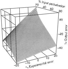
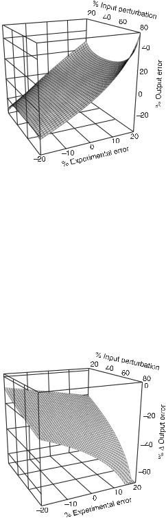
Figures 12.2 and 12.3 show the error of the evaluated self-replication rate constant as a function of the experimental error and of the variation of the input flux for emulated experiments of type (a) and (b), respectively. In the case of emulated experiments of type (a) for which the evaluation of the rate constant is based on linearized kinetic equations, the error of the evaluated rate constant depends strongly on the variation of the input perturbation. The range of the final output error (−40%,+10%) is distorted in comparison with the range of the experimental error (−20%,+20%). For small values of the input perturbation, between 20% and 40%, the output error is surprisingly small—between 10% and 0%. As the input perturbation increases, the accuracy of the method deteriorates rapidly and for large perturbations the output error is almost twice as big as the experimental error. For the emulated experiments of type (b), where the rate coefficient is evaluated from our exact response law (12.105) without linearization, the situation is different. For input perturbations between 20% and 70% the error of the evaluated rate coefficient has about the same range of variation as the experimental error (−20%,+20%) and does not depend much on the size of the perturbation. For very large input perturbations, between 70% and 80%, the output error increases abruptly. In fig. 12.4 we show the difference of errors of the evaluated self-replication

Fig. 12.2 The error of the evaluated selfreplication rate constant (output error) versus the experimental error and the input perturbation for an emulated response experiment of type (a). The rate constant is evaluated by using a linearized evolution equation. The range of the output error (−40%, +10%) is strongly distorted in comparison withy the range of the experimental error (−20%, +20%). The output error varies greatly with the perturbation size: for large perturbations it is about twice the experimental error, whereas in other regions there is error compensation. (From [11].)

Fig. 12.3 The error of the evaluated selfreplication rate constant (output error) versus the experimental error and the input perturbation for an emulated response experiment of type (b). The rate constant is evaluated from the susceptibility function computed from the exact response law. The range of the output error is about the same as the range of the input error for input perturbations between 20% and 70% and does not depend much on the size of the perturbation. For input perturbations between 70% and 80% the output error is bigger. (From [11].)

rate constant (output error) evaluated from emulated experiments of type (a), with linearization, and type (b), without linearization, respectively. We notice that the two approaches lead to different results: the evaluated values of the rate coefficient are different even for small experimental errors and input perturbations. The biggest differences occur for large perturbations, because for large perturbations the linear approach is very inaccurate.

The physical interpretation of the results presented in figs 12.2–12.4 is the following. Like any autocatalytic processes, chemical reactions (12.123)–(12.125) lead to saturation effects due to the balance between self-replication and consumption (disappearance) processes. The saturation effects are nonlinear and as a result the experimental errors propagate nonlinearly, which explains the error distortion displayed in fig. 12.2.

Fig. 12.4 The difference of errors of the evaluated self-replication rate constant (output error) evaluated from emulated experiments of type (a), with linearization, and type (b), without linearization, respectively. The figure shows that the variations of the input perturbation and of the experimental error have a different effect on the two types of response methods. The biggest difference occurs for large perturbations, because for large perturbations the linear approach is very inaccurate. (From [11].)

196 DETERMINATION OF COMPLEX REACTION MECHANISMS

Even though the analysis of the process is based on linear equations, the intrinsic dynamics of the process is nonlinear and the errors are distorted. This error distortion interferes with the numerical errors due to linearization, resulting in fig. 12.2. In some regions these two errors can have opposite signs, resulting in error compensations, whereas in other regions the two errors add up, leading to large output errors. For neutral response experiments of type (b), linearization is not necessary for the evaluation of the rate coefficients and the most important source of errors are the experimental errors. This is the reason why the output error follows closely the input error and there is almost no error compensation or error amplification.

Numerical errors do, however, have some influence in the case of neutral experiments, especially for very large input perturbations. If the input flux contains a very large fraction of marked (labeled) compound, the dynamics of the marker is close to saturation and in this area small variations of the input flux lead to relatively large variations in the output, which produces numerical errors in the deconvolution of eq. (12.105). This effect explains the spike in fig. 12.3 for large perturbations. It follows that, even for response experiments of type (b), it is not recommended to use very large input perturbations. Nevertheless, it seems that the admissible input perturbations that produce reasonable results are much larger than the admissible perturbations for experiments of type (a) for which the analysis is based on linearized evolution equations.

We have also emulated experiments that involve the measurement of more than one flux, in order to determine the cumulative effect of errors produced by more than one measurement. We have considered the evaluation of two transformation constants. Unfortunately in this case the results cannot be easily represented as compact, 3D graphs. The analysis revealed a complication typical for multiple flux measurements: experimental errors may lead to an apparent violation of the law of mass conservation. We considered only errors that preserve the mass conservation. We noticed the same qualitative features as in the case of the self-replication constant. For experiments of type (a), with linearization, in general there is a distortion of the range of the output error compared to the range of the input error. We have also noticed error compensation and error accumulation; in some cases they exist in more than one region and alternate, one compensation region followed by an accumulation region. Sometimes the amplification error tends to be very large; we have noticed output ranges of the error 4–5 times larger than the maximum range of the measurement errors of the fluxes. The emulated experiments of type (b) are also affected by the cumulative measurement errors in a complicated way. There is a region where the range of the output error is about the same as the maximum range of the input experimental error. However, the maximum admissible input fluxes are smaller than in the case of a single response experiment; in our simulations it varied from approximately 60–65% (compared to 80% for single response experiments) to 35–40%.

Although the detailed results of our computations are probably model specific, we believe that the qualitative features discussed above have general significance. It is likely that the analysis of a response experiment based on linearized equations will lead to error compensation in some regions and to error amplification in other regions. The nonlinear saturation effects occurring in our model are likely to exist even though the autocatalytic steps are missing. For example, enzymatic reactions display saturation effects due to the limited supplies of the enzymes. The error compensation is as harmful as error amplification because in general it is impossible to predict a priori where it occurs.

Concerning the neutral response experiments for which the linearization results are not necessary, it is likely that they lead to better results than the experiments of type (a) for which the analysis is based on the linearization of the kinetic equations. However, even for neutral experiments the use of very large input perturbations requires caution, owing to the proximity to saturation, which results in numerical errors. Multiple measurements with large errors introduce further complications which reduce the potential value of experiments of type (b), without linearization, for large perturbations.

In conclusion, the linearization of the evolution equations for the analysis of chemical and biochemical networks is unpredictably limited. For the linearization to be valid it is necessary to use small perturbations, for which the experimental errors are very large. In the papers that have appeared on this subject, insufficient (or no) attention has been given to error accumulation and propagation [25]. The response approaches developed here avoid linearization and hence are to be preferred.

12.6Response Experiments for Reaction–Diffusion Systems

Our response approach can be extended to inhomogeneous, space-dependent systems. Such a generalization is of interest not only for biochemistry and molecular biology, but also for population biology. In the following we consider a generalized approach, which can be applied to various problems in physics, chemistry, and biology. For simplicity we assume that there is only one fragment in each carrier. We consider a complex system made up of different types of individuals (species) which can be atoms, molecules, quasiparticles, biological organisms, etc. The different types of individuals interact with each other and at the same time are involved in motion, which can be described by transport operators local in time.

We denote by ρu(r; t), u = 1, 2, . . . , the concentrations of the different species at position r and time t, expressed in numbers of individuals per unit volume, and assume that the rate of change of the species u, Ru(t), can be expressed as a local, nonlinear, function of the composition vector ρ(r; t) = [ρu(r; t)]u=1,2,..., and of time t:

where Ru+(ρ(r; t)) ≥ 0 and Ru−(ρ(r; t)) ≥ 0 are formation and consumption rates, respectively. The transport of the different species can be described by transport operators Lu . . . , which are local in time and generally nonlocal in space. In this chapter we limit ourselves to transport operators of the “master” type:

Lu . . . = . . . Wu ρ(r ; t), r → r dr − . . . Wu ρ(r; t), r → r dr (12.128)

r

where Wu ρ(r ; t), r → r are concentration-dependent transition rates. The operators describe the regular (Fick) as well as anticrowding diffusion processes as particular cases. The evolution equations of the process are:

where Ju+(r, t) is the input flux of species v, which is generally spaceand timedependent and can be controlled by the experimenter, and Ju−[ρ(r, t)] is the output

198 DETERMINATION OF COMPLEX REACTION MECHANISMS

flux of species u which is assumed to depend on the composition vector. Each species u = 1, 2, . . . may exist in two different forms, “marked” and “not marked,” and both forms fulfill a “neutrality condition” similar to the one introduced for homogeneous systems, that is, their kinetic and transport properties are identical.

In chemical kinetics a “marked species” can be a molecule containing a radioactive isotope and we neglect the kinetic isotope effect. In fluid mechanics a “marked species” can be a colored fluid for which the hydrodynamic properties (density, viscosity, diffusion coefficients) are the same as the ones of the main fluid. In population genetics a “marked species” can be an individual carrying a neutral mutation, and for which the main functions describing the vital statistics (natality and mortality functions, diffusion coefficients) are the same as in the case of a nonmutant individual. In the following we denote by ρu(r, t) and ρu (r, t) , u = 1, 2, . . . , the concentrations of the “not marked”

and “marked” species, respectively, and by ρu (r, t) = ρu(r, t)+ρu (r, t), u = 1, 2, . . . , the total concentrations of the species.

At the beginning of the experiment the system contains only “not marked” species. The system need not be but may be in a stationary state. The experiment consists in varying the ratios

between the input fluxes of Ju+(r, t), the “marked” compounds, and the total input fluxes, Ju+ (r, t), with the preservation of the total input fluxes Ju+ (r, t). We record the response to these variations, the fractions

system, expressed by the fractions αu(r, t), and the response of the system, expressed by the fractions βu(r, t).

We assume the existence of generalized “neutrality conditions” [8,11], in the form of scaling laws, which connect the kinetic and transport laws for the whole system to the

Equations (12.132) express the fact that the “marked” and “not marked” species contribute equally to the transport process. We assume that the output fluxes, Ju− [ρ (r, t)], are expressed by kinetic laws, and thus they also obey a scaling condition similar to eq. (12.132):

×Wu ρ (r ; t)+ρ(r ; t),r → r dr, u = 1,2,....

The response experiment can be described in terms of two sets of nonlinear evolution equations of the type (12.129), one set for the labeled concentration vector ρ (r; t), and the second set for the total concentration vector ρ(r; t) + ρ (r; t), respectively. The transport and reaction rates in these two sets of evolution equations are connected to each other by means of the neutrality conditions (12.132)–(12.134). Together with suitable initial and boundary conditions, these two sets of evolution determine the time and space dependence of the total concentrations of the different species, as well as the concentrations of the marked species. Despite their nonlinearity, these two sets of evolution equations lead to a linear response law, which relates the excitation functions αu(r, t) to the response functions βu(r, t). By using the neutrality conditions (12.132)– (12.134) and the definitions (12.130)–(12.131) for the excitation and response functions, after lengthy algebraic manipulations, the two sets of nonlinear evolution equations lead to a set of linear integro-differential equations, which relate the responses βu(r, t) to the excitations αu(r, t). By representing the solution of this set of linear equations in terms of Green functions, we come to a generalization of eq. (12.105):

where the spaceand time-dependent susceptibility function χuu (r , t → r, t) is nonnegative and obeys the normalization condition:

It is possible to show that the susceptibility function has a physical interpretation, similar to the one existing for homogeneous systems. It is related to the probability density

(12.137)

that a species u which leaves the system at time t and position r entered the system as the species u , spent in the system a residence time between τ and τ + dτ, with τ = t − t , and has a displacement vector between r and r + d r, with r = r − r . We have

According to eq. (12.138) the physical significance of the linear response law (12.135) is straightforward: it expresses the contribution to the output fraction of marked species entering the system in different forms u , at different initial positions r and different initial times, t = t − τ. The weight function (susceptibility function)

are deviations of the individual rate and transport coefficients from the corresponding average values,

are transport (hydrodynamic) speeds and expansion coefficients attached to different population fractions,

are the components of the rates of change of the population fractions due to the individual variations of the rate and transport coefficients, and γ = (γ1, γ2, . . .) is the vector of population fractions.

We notice that, even though the different species are undergoing slow, diffusive motions, the corresponding population fractions move faster: in the evolution equations (12.141) there are both diffusive terms as well as convective transport (hydrodynamic) terms depending on the transport speeds vu given by eqs. (12.145). According to eqs. (12.145) these transport speeds are generated by the space variations of the total population density and have the opposite sign of the gradient of the total population densities. For a growing population the population cloud usually expands from an original area and tries to occupy all space available. The population density decreases toward the edge of the population cloud; thus the population gradient is negative and the transport velocities are positive, oriented toward the directions of propagation of the population cloud. It follows that the cause of enhanced transport of the species fractions is the net population growth. Since the gradient tends to increase toward the edge of the population wave, an initial perturbation of the species fractions generated in the propagation front of the population has a good chance of undergoing enhanced transport and spreading all over the system. An initial perturbation produced close to the initial area where the population originates has a poor chance of undergoing sustained enhanced transport.

It is important to clarify the mathematical and physical significance of the hydrodynamic transport terms (vu γu) in eqs. (12.141). From the mathematical point of view the terms (vu γu) emerge as a result of a nonlinear transformation of the state variables, from species densities to species fractions. The physical interpretation of the transport terms (vu γu) depends on the direction and orientation of the speed vectors: for expanding populations vu are generally oriented toward the direction of expansion of the population cloud, resulting in enhanced transport. For shrinking population clouds the terms (vu γu) lead to the opposite effect, that of the transport process slowing down.

In general, different population fractions have different propagation speeds. An interesting particular case is that for which the replication and disappearance rate coefficients

202 DETERMINATION OF COMPLEX REACTION MECHANISMS

and the diffusion coefficients are the same for all species and depend only on the total population density ρu±(x) = ρ±(x), Du = D. Moreover, we assume that the transformation rates are constant, kuv (x) = kuv . This type of condition is fulfilled in chemistry by tracer experiments, for which the variation of the rate and transport coefficients due to the kinetic isotope effect can be neglected [18]. Similar restrictions are fulfilled in population genetics, in the case of neutral mutations, for which the demographic and transport parameters are the same for neutral mutants and nonmutants, respectively [12]. For neutral systems the evolution equations turn into a simpler form:

where µ(x) = ρ+(x) − ρ−(x) is the net production rate of the total population. We notice that the total population density obeys a separate equation, which is independent of the species fractions, and the evolution equations for the fractions become linear.

Now we can investigate the problem which suggested the present research, the geographical spreading of neutral mutations in human populations [12,27]. We consider a growing population which diffuses slowly in time and assume that the net rate of growth is a linear function of population density, µ(x) = L(1 − x/x∞), where L is Lotka’s intrinsic rate of growth of the population. We assume that, at an initial position and time, a neutral mutation occurs and afterwards no further mutations occur. We are interested in the time and space dependence of the local fractions of the individuals, which are the offspring of the individual that carried the initial mutation. The ultimate goal of this analysis is the evaluation of the position and time where the mutation originated from measured data representing the current geographical distribution of the mutation. We limit our analysis to one-dimensional systems, for which a detailed theoretical analysis is possible. Equations (12.146)–(12.147) become

where γ is the local fraction of mutants. Equation (12.148) for the total population growth is the well-known Fisher equation [28] which has solitary solutions.

Two different solitary wave solutions for eq. (12.148) have been derived in the literature. There is an asymptotic solution developed by Fisher and others [28] and an exact solution derived by Ablowitz and Zeppetella [29]. The asymptotic solution gives an excellent representation of the population wave from the top saturation level to the front edge where the total population tends to zero. The usefulness of the exact solution of Ablowitz and Zeppetella has been questioned in the literature [28] because, although exact, it does not represent all possible solutions and the most relevant solutions may not be represented by it. In the following we consider only the Fisher solution, which is biologically significant [12]. For the application of the Ablowitz and Zeppetella solution,

For a mutation that occurs at the very edge of the total population wave, x 0, the transport speed is equal to the speed of propagation front, v = c; the motion of two waves, for the total population and the mutation, is synchronized.

Now we can address the problem of determining the position where a mutation originates. The probability density P (r, t) of the position of the center of gravity of the mutant population can be roughly estimated by normalizing the mutant gene frequency:

P (r, t) γ (r, t)/ γ (r, t)dr (12.153)

By applying eq. (12.153) we obtain a Gaussian distribution for the position r of the center of gravity of the mutant population both for the diffusive regime and for the enhanced transport:

P (r, t) [4π D (t − t0)]−1/2 exp − (r − r0 − veff (t − t0))2/[4D (t − t0)]

(12.154)

where r0 and t0 are the initial position and time where the mutation occurred and veff is an effective transport rate. In eq. (12.154) we have veff 0 for diffusive transport, x x∞, and veff c for the enhanced transport, x 0. Although for intermediate cases between these two extremes the probability density P (r, t) is generally not Gaussian, eq. (12.154) can be used as a reasonable approximation, where the effective propagation speed veff has an intermediate value between zero (diffusive transport) and the maximum values for enhanced transport corresponding to the two solutions of the Fisher equation. Under these circumstances the average position of the center of gravity of the mutant population increases linearly in time. From eq. (12.154) we obtain:

r(t) = rP (r, t)dr = r0 + veff (t − t0) (12.155)

If we examine the current geographical distribution of a mutation it is hard to estimate the value of the population density x at the position and time where the mutation originates. Under these circumstances it makes sense to treat x as a random variable selected from a certain probability density p(x). The only constraints imposed on p(x) are the conservation of the normalization condition p(x)dx = 1, and the range of variation, x∞ ≥ x ≥ 0. By using the maximum information entropy approach, we can show that the most unbiased probability density p(x) is the uniform one:

204 DETERMINATION OF COMPLEX REACTION MECHANISMS

where h(x) is the Heaviside step function. By considering a large sample of different initial conditions, veff can be evaluated as an average value:

veff = v(x)p(x)dx (12.157)

where v(x) is given by eqs. (12.151). We have

For the estimation of the initial position of a mutation it is useful to consider the ratio

where r(tL) is the position of the limit of expansion, tL is the time necessary for reaching the limit of expansion, r(tL) is the position of the center of gravity of the mutant population for t = tL, and r(t0) = r0 is the position where the mutation originates. In eq. (12.159) both r(tL), the position of the limit of expansion, and r(tL) , the current average position of the center of gravity of the mutant population, are accessible experimentally. It follows that, if the ratio ζ can be evaluated from theory, then r(t0) = r0, the point of origin of the mutation, can be evaluated from eq. (12.159). By taking into account that the total population wave moves with the speed c and that the average center of gravity moves with the speed veff , we have

From eqs. (12.157) and (12.160) it follows that ζ = 2, a value that is in good agreement with the numerical simulations of Edmonds et al. [27], which lead to ζ = 2.2. The difference of 0.2 between theory and simulations is due to the random drift, which was taken into account in the simulations but is neglected in our theory. By including the random drift, our theory provides information about the details of the motion of the propagation front [12].

In conclusion, we have shown that the neutral response approach can be extended to inhomogeneous, space-dependent reaction–diffusion systems. For labeled species (tracers) that have the same kinetic and transport properties as the unlabeled species, there is a linear response law even if the transport and kinetic equations of the process are nonlinear. The susceptibility function in the linear response law is given by the joint probability density of the transit time and of the displacement position vector. For illustration we considered the time and space spreading of neutral mutations in human populations and have shown that it can be viewed as a natural linear response experiment. We have shown that enhanced (hydrodynamic) transport due to population growth may exist and developed a method for evaluating the position of origin of a mutation from experimental data.