Oscillatory Reactions

126 DETERMINATION OF COMPLEX REACTION MECHANISMS

Autocatalysis involves a pathway of two species, the bromic acid HBrO2, and a radical BrO•2, where the bromic acid reacts with bromate to produce two molecules of the radical, which in turn react with a metal ion catalyst such as Ce3+ to produce two molecules of bromic acid [17]. So the overall process

HBrO2 + BrO−3 + 2Ce3+ + 3H+ → 2HBrO2 + 2Ce4+ + H2O

provides net stoichiometric production of bromic acid that makes the autocatalysis possible. More technical conditions for the occurrence of autocatalytic instability are provided by stability analysis of a steady state in association with various theories of reaction networks [10,18]. Later in this chapter we shall use a particular approach called the stoichiometric network analysis [10].

Since the main reactants, bromate and malonic acid, are in surplus, inhibition and negative feedback in the BZ reaction are quite different from that in the previous example of thermokinetic oscillations. Inhibition is provided in part by a direct decomposition of HBrO2 (analogous to heat removal in the previous example) but mainly by a chain of reactions of oxidized ion catalyst with brominated malonic acid (BrMA), summarized as

Ce4+ + qBrMA → Ce3+ + qBr− + products

which regenerates the catalyst and provides bromide ions, Br−. The overall stoichiometric coefficient q is somewhere in the range 1/2 < q < 1 depending on external conditions. Bromide ions in turn control the autocatalytic species HBrO2:

Br− + HBrO2 + H+ → 2HOBr

Further reactions (omitted here) produce free bromine that takes part in another sequence of reactions that brominate malonic acid.

The pathway from Ce4+ to Br− is the key to negative feedback on HBrO2, which helps to remove this species after being accumulated due to autocatalysis. However, different roles are associated with the two species: while Br− is an inhibitor that directly removes HBrO2, Ce4+ is a controlling species that provides a delay allowing the autocatalysis to advance considerably before inhibition by Br− causes the concentration of HBrO2 to drop; hence oscillations may appear. As before, proper time scales of reaction steps are necessary for oscillations to appear. Clearly, this example of isothermal oscillations is more involved than the thermokinetic one. In particular, there are three main (or essential) types of variables rather than two; this observation prompts for a classification of oscillatory reaction mechanisms—one of the main topics of this chapter.

Reactions along the autocatalytic pathway are very fast; typical time scales are fractions of a second. Likewise, the reactions removing the autocatalytic species are rapid, whereas the reaction of a transport process controlling the negative feedback (inflow of the reactant in the thermokinetic example, and conversion of BrMA to Br− in the BZ reaction) is slower by one or more orders of magnitude. This typically produces rather sharp oscillatory peaks and in extreme cases results in a series of spikes interconnected by a recovery phase of relative quiescence; the period of oscillations is typically in the range from tens to hundreds of seconds. The range of concentrations is also varied. The autocatalytic and inhibitory species tend to oscillate within several orders of magnitude in their concentration, whereas the species controlling the negative feedback

typically has a smaller span. Still other species may have yet smaller amplitude and may be buffered with no suppression effect on oscillations (nonessential species).

There are many examples of oscillating chemical reactions provided in the literature [1,19–21]. But the main realm of oscillatory behavior is in biochemical reactions that take place in vivo [22–27]. Oscillating biochemical reactions are used by cells as pacemakers [28], means of signaling and information processing [29], metabolic control such as maintaining stable energy supply [30], and output of products [31]. The efficiency of oscillatory reactions is discussed briefly in section 10.3. One example, glycolytic oscillations, has been examined throughout this book. Other examples include repeated firings of neurons, bursting in pancreatic cells, pacemaker cells in the heart, oscillations of calcium ions in cytosol, proton pumps, muscle contraction, and so on (see, for example, Keener and Sneyd [32] and Fall et al. [33]). Among those, intracellular [Ca2+] spiking [34,35] is of particular interest, since calcium ions are critically important for many cellular functions including muscle contraction, cardiac electrophysiology, hormone secretion, and others. Oscillations also play an important role in the transcriptional control in genetic networks [36,37].

Much research on oscillatory reactions has been concerned with the complex reaction mechanisms, with many variables and many elementary steps, that give rise to temporal oscillations of concentrations of species in the mechanism. Hypothesized reaction mechanisms have been tested by comparing calculated periods (frequencies), amplitudes, and the shape of temporal variations of oscillating species with experimentally observed behavior. This is an important but frequently not stringent test; also such comparisons are usually not suggestive of improvements in a proposed reaction mechanism. In the last few years, a series of theoretical studies and suggestions of new types of experiments have provided more stringent tests of a proposed mechanism and have led the way to a strategy for formulating reaction mechanisms, based on operational prescriptions, that is, a set of experiments. In this chapter we outline these developments. In section 11.2 we describe several necessary theoretical concepts and constructs of oscillatory reactions. In section 11.3 we list and briefly describe a series of experiments showing what information about the reaction mechanism can be deduced from each type of experiment. We also give examples of the application of these techniques to various experimental systems. In section 11.4 we illustrate the strategy of carrying out the experiments described in section 11.3 on two experimental systems: the horseradish peroxidase oscillatory reaction and the chlorite–iodide reaction.

We focus here on strategies of formulating reaction mechanisms of oscillatory chemical reactions in open (flow-through) and closed (oscillating for a limited time) homogeneous systems with no spatial gradients (either because of stirring or because of relatively fast diffusion in small cell-sized systems).

11.2Concepts and Theoretical Constructs

A homogeneous oscillatory chemical reaction in a closed system is described by a set of ordinary differential equations

128 DETERMINATION OF COMPLEX REACTION MECHANISMS

one for each of the species. Here Xi is the concentration of species i and the net reaction rate Ri for species i is obtained as a sum over contributing rates from a reaction mechanism consisting of elementary steps by use of mass action kinetics (see section 11.2.4). In an open system (a continuous-flow stirred tank reactor—CSTR) terms are added for inflows and outflows, giving

dXi

(11.2)

dt

where k0(Xi0 − Xi ) is the term due to inflow and outflow of the ith species, k0 is the reciprocal residence time (or flow rate), and Xi0 is the input concentration of the ith species.

the JMEs give useful information about both the stability of the stationary state and the connectivity among the species in the reaction mechanism of the system. The time evolution of the deviation δX from the stationary state is given in terms of the eigenvalues λk and eigenvectors wk = (w1k , . . . , wnk ) (where k = 1, . . . , n) of the Jacobian matrix,

k=1

where the numbers ak specify the initial deviation at t = 0. The stability is determined by the eigenvalues, namely, if real parts of all λk ’s are negative, then the stationary state is stable.

Tyson [38] classified destabilizing processes in chemical reaction systems according to mathematical relations among the JMEs. He distinguished direct autocatalysis,

which includes product activation and substrate inhibition; indirect autocatalysis, as seen in competition, symbiosis, and positive feedback loops; and negative feedback loops. Luo and Epstein [19] extended Tyson’s classification, emphasizing the important interplay between them in oscillating chemical systems. They distinguished three distinct types of negative feedback: coproduct autocontrol, double autocatalysis, and flow control. Chevalier et al. [7] presented new experimental strategies for measuring JMEs at a stationary state of a complex reaction and a discussion of how JMEs may be used to construct a reaction mechanism (see section 11.3.7).

11.2.2 Bifurcation Analysis

A given reaction mechanism may have various dynamic regimes displayed in the space of variables (phase space), corresponding to different regions in the space of constraints or parameters. Variables are the quantities Xi in eqs. (11.2) such as concentrations of reactants, intermediates, and products, and other dynamical quantities, such as temperature in nonisothermal systems. Constraints are imposed, experimentally controllable conditions, such as influx of reactants into an open reaction system, whereas parameters specify properties of the system; examples of parameters are rate coefficients.

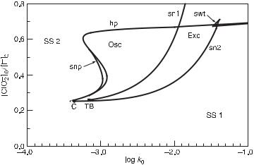
The ranges of various dynamic regimes are often displayed in a two-dimensional (2D) bifurcation diagram. An example is given in fig. 11.1, obtained by calculation [5] from a model of the chlorite–iodide reaction [39,40]; the 2D space of constraints in

Fig. 11.1 Two-dimensional bifurcation diagram calculated by continuation from the Citri–Epstein mechanism for the chlorite–iodide system. Plot of 2D space of constraints is chosen to be the ratio of input concentrations, [ClO−2 ]0/[I−]0, versus the logarithm of the reciprocal residence time, log k0. Notation: SS1, SS2, region of steady states with high [I−] and low [I−], respectively; Osc, region of periodic oscillations; Exc, region of excitability; sn1, sn2, curves of saddle-node bifurcations of steady states; hp, curve of Hopf bifurcations; snp, curve of saddle-node bifurcations of periodic orbits; swt, swallow tail (a small area of tristability); C, cusp point; TB, Takens–Bogdanov point (terminus of hp on sn1). (From [5].)

130 DETERMINATION OF COMPLEX REACTION MECHANISMS

the diagram is chosen to be the ratio of input concentrations, [ClO−2 ]0/[I−]0, versus the logarithm of the reciprocal residence time, log k0. Several regions with different dynamics are shown: two different stable stationary states; a region of periodic oscillations; a region of two coexisting stable stationary states; and a region where one stable stationary state is excitable (i.e., sensitive to small but superthreshold perturbations that evoke a single large-amplitude peak). In addition, there is a small region of a stable stationary state coexisting with oscillations, and a small region of three coexisting stable stationary states. The various regions are separated by boundaries corresponding to different types of transitions or bifurcations: a Hopf bifurcation, separating stationary states from oscillations; and saddle-node bifurcations of stationary states/periodic oscillations, indicating where a pair of stationary states/periodic orbits merge and disappear.

As a complement, a one-dimensional (1D) bifurcation diagram is a plot of one constraint (or parameter) versus a norm or another characteristic of the displayed dynamic regime. The norm can simply be one of the dynamic variables (time averaged in the case of oscillatory regimes) or a combination of more variables, for example, a Euclidean

#

This diagram adds information on the space of variables at the expense of the space of constraints/parameters, the dimension of which is decreased by one. Figure 11.2 shows a 1D bifurcation diagram calculated for the same model used to generate the 2D diagram in fig. 11.1. Here the constraint log k0 is retained, where as [ClO−2 ]0/[I−]0 is fixed. The diagram indicates various branches of dynamical regimes: stable steady states as solid lines, unstable steady states as dashed lines, and periodic orbits (or limit cycles) as small dashed lines (this branch is mostly stable, only the part between HP and snp is unstable). From this, ranges of k0 can be identified over which stationary states and

Fig. 11.2 One-dimensional bifurcation diagram calculated by continuation from the Citri–Epstein

#

mechanism for the chlorite–iodide system. The norm for the steady states is i Xi2, and for the

#

unstable steady states; small dashed lines and po, branch of periodic solutions; other notation corresponds to fig. 11.1. (From [5].)

periodic oscillations represent unique stable dynamical regimes, and where the system is multistable. In this case, multistability occurs where the branches of stable SS2 and stable periodic orbits overlap.

Theoretical background for bifurcation analysis can be found, for example, in Guckenheimer and Holmes [41]; calculations of 1D and 2D bifurcation diagrams can be done by continuation methods [42–45]. 2D bifurcation diagrams typically contain a cusp-shaped region of multiple stationary states and essentially delineate regions of oscillatory and nonoscillatory behavior, as well as regions of excitability and regions of bior multistability between stationary states or other dynamic regimes. A predominantly occurring structure called the cross-shaped diagram [46] involves the cuspshaped region bounded by a curve corresponding to a saddle-node bifurcation, and a curve corresponding to a Hopf bifurcation, which makes an α-shaped loop surrounding the cusp point, intersects itself within the cusp-shaped region, and touches the saddlenode curve in two endpoints (Takens–Bogdanov points). Thus the oscillatory region extends beyond the tip of the cusp; bistability of stationary states is confined to the interior of the cusp and excitability occurs in between. This highly symmetric structure (see, e.g., fig. 11.8c) may not always be present; in many cases the self-intersection is missing (as in fig. 11.1) or there are two separate branches of the Hopf bifurcation (as in figs. 11.8d–f).

Predictions of proposed reaction mechanisms are tested against experiments. The details of bifurcation diagrams are useful in seeing the complexity of dynamic regimes of chemical reactions and in providing a series of predictions on dynamic regions and on types of bifurcations to be tested against experiments. Clarke and Jiang [47] provided a method for deriving approximate equations for Hopf and saddle-node bifurcation surfaces of chemical reaction networks, using the methods of stoichiometric network analysis (SNA) to assess the effects of adding or deleting particular reactions on the character of the bifurcation of the network. The methods of SNA will be discussed in more detail in the next section in connection with a categorization of oscillatory reactions.

Some features of bifurcation diagrams are universal, in the sense that if they occur in reaction mechanisms, these features do not distinguish one mechanism from another; other features are specific to a particular reaction mechanism. For example, the increase in amplitude of oscillations of concentrations near a supercritical Hopf bifurcation with a varying constraint is a universal (square root) function. On the other hand, the tilt of the cusp-shaped region in an inflow concentration/flow rate bifurcation diagram is specific to a given species in an oscillatory mechanism, as well as the direction of a transition between high and low stationary state concentration for a given species in a 1D bifurcation diagram. There is an inherent appeal in universality, particularly for mathematicians and physicists. For chemists with their concern for reaction mechanisms, universal features give some general information, such as the presence of a feedback in the reaction mechanism with a Hopf bifurcation; however, specific features may be necessary to distinguish among competing suggested mechanisms.

11.2.3 Role of Species in Oscillatory Reactions

Eiswirth et al. [1] proposed a categorization of chemical oscillators. First, a distinction is made between nonessential and essential species. If the concentration of a nonessential species is held constant, oscillations continue. In contrast, if the concentration of an essential species is fixed, oscillations cease. In analyzing the core mechanism of a

132 DETERMINATION OF COMPLEX REACTION MECHANISMS

chemical oscillator, nonessential species may be neglected or considered as parameters, which simplifies the problem under consideration. The categorization is based on experiments, detailed later, that lead to identification of essential chemical species and their roles in producing the instability leading to oscillatory behavior, and to the connectivity of these species in the elementary steps of the mechanism.

Three types of nonessential species are distinguished. Nonessential species of type A are those that react to produce essential species but do not interact (or only weakly) with other species; type A species can be omitted as dynamic variables and modeled as inflows of the essential species they produce. Nonessential species of type B are inert (or nearly inert) products of the reactions, since, in the limiting case of irreversible reactions, they do not act as reactants anywhere in the network (or do so to a negligible extent); they can thus be left out from the mechanism without (significantly) affecting any other species. Nonessential species of type C react with at least one essential species and may take part in several reactions. Typically, the concentration of type C species may be large and nearly constant; hence buffering the species will have no suppressing effect on oscillations.

In mathematical terms, this classification can be related to the eigenspaces of the Jacobian matrix evaluated at an unstable stationary state surrounded by a stable limit cycle near the supercritical Hopf bifurcation. This bifurcation is characterized by a pair of pure imaginary eigenvalues of the Jacobian matrix. The emerging (small) limit cycle is an ellipse embedded in a plane within the phase space spanned by two eigenvectors that are associated with the pair of bifurcating eigenvalues (center eigenspace). If this plane is perpendicular (or nearly so) to the axis of a particular species, then the limit cycle projects onto this axis as a point (or a small interval), and consequently this species will have (nearly) zero amplitude of oscillations. This is exactly what characterizes type A and type C species. It is convenient to use relative amplitude obtained by scaling the oscillatory amplitude of the species with its stationary value. The remaining (n − 2) eigenvalues are stable and the corresponding eigenvectors span a stable eigenspace of dimension (n − 2); for three variables, this eigenspace is simply a straight line. If the axis of a species intersects the stable eigenspace at a nonzero angle, then perturbing the oscillations at a specific phase with a specific amount of that species will hit the stable eigenspace and the system will be driven to the stationary state—in other words, the oscillations are quenched [48] (in practice only temporarily, since the stationary state is unstable and ever-present fluctuations will eventually reinstate the oscillations). However, if the axis runs (nearly) parallel with the stable eigenspace, then the size of the quenching perturbation (called the quench vector) would be (nearly) infinite. This is the characteristic of type B and type C species. Therefore relative amplitudes and quench vectors discriminate between all types of nonessential species, and separate them from essential species, as shown in table 11.1. For other ways of determining nonessential species see Stemwedel et al. [2].

The roles of essential species in mechanisms of chemical oscillators are defined as:

1.Autocatalytic or cycle species (those involved in a reaction in which an increase in the concentration of a species increases the rate of production of that species), denoted X.

2.Exit species (those exerting direct inhibitory effect on the cycle species by reacting with it to produce nonessential species or essential species other than X), denoted Y.

Table 11.1 Limiting values of relative amplitudes and quench vectors of nonessential and essential species

3.Feedback species (those exerting indirect inhibitory effect on the cycle species by providing negative feedback on the autocatalytic cycle), denoted Z.

4.Recovery species (those that take part in reactions allowing the autocatalysis to recover), denoted W.

Not all of these roles are necessary in every category of oscillator.

11.2.4 Stoichiometric Network Analysis (SNA)

In order to discuss the categorization of oscillators set forth by Eiswirth et al. [1], we must first review some of the concepts set out by Clarke [10] in his development of the SNA. Assume that there are m species taking part in r chemical reactions so that n species, n ≤ m, are entering at least one of the reactions:

nm

where νijL ≥ 0 and νijR ≥ 0 are, respectively, the left-hand and right-hand stoichiometric coeffcients of species Xi in reaction Rj . The first n species are assumed to be reactants or intermediates and the remaining m − n are inert products, which can be left out from further consideration (these are “ideal” type B species). Let S = !νijR − νijL" be the (n × r) stoichiometric matrix, X = (X1, . . . , Xn) the vector of the chemical species concentrations, and V (X) = (V 1(X), . . . , V r (X)) the vector of reaction rates. The

chemical equations (11.7) together with the vector function V (X) define the mechanism of the reaction, also called a stoichiometric network. Only the concentrations of reactants and intermediates are dynamical variables for which independent dynamical equations can be written. The time evolution of X in a flow-through system at constant temperature in a well-stirred reaction cell of constant reaction volume can be, according to eqs. (11.2), rewritten in vector notation as

where X0 = (X01, . . . , X0n) is the vector of feed concentrations for each species and k0 is the flow rate (or reciprocal residence time). The inflow and outflow terms can be formally treated as zeroth and first-order pseudoreactions, respectively, and are conveniently included in an extended reaction rate vector V (X) = (V , k0X0, k0X) having nonnegative components. Accordingly, an extended stoichiometric matrix is S = [S, I, −I ], where I is an identity matrix. Then F(X) is simply expressed as SV(x).

134 DETERMINATION OF COMPLEX REACTION MECHANISMS

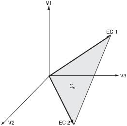
Fig. 11.3 Three-dimensional reaction rate space spanned by the axes V1, V2, V3 with a two-dimensional current cone Cv spanned by two extreme currents EC1 and EC2. The shaded bounded region of the cone is obtained by applying the normalizing condition

K 1 αk Ek ≤ 1. (From [5].) k=

A stationary state Xs satisfies the equation SV(X) = 0. Hence Vs = V (Xs ) is contained in the null space of S. Moreover, all components of S must be nonnegative numbers, which narrows the set of all possible stationary reaction rate vectors Vs (the currents in SNA terminology) to an open, convex, dr -dimensional cone, dr = r − rank(S), in the space of all V ’s. The edges of this steady-state cone represent sets of steady states that have minimum possible nonzero V ’s admitted by eq. (11.8), and uniquely define a set of major subnetworks (or extreme currents) of the mechanism. In general, the number K of such subnetworks equals at least the dimension of the cone, K ≥ dr . An example of a current cone is shown in fig. 11.3.

extreme currents (such a decomposition is, however, not unique if K > dr ). If the Ek ’s

of the steady-state cone, d = 2, . . . , dr − 1. Hence there is a hierarchy of subnetworks associated with edges and faces of the steady-state cone that may be used as simplified models instead of the full network. The identification of the edges and faces is useful when examining the stability of the (sub)network at a stationary state Xs . The Jacobian matrix J of eq. (11.8) at Xs is

if the reaction rates obey power law kinetics, then κij is independent of Xs . Thus a reparametrization of eq. (11.8) is suggested such that Xs1, . . . , Xsn and α1, . . . , αK are new parameters. If power law kinetics is in effect, the stability of the current Vs is indicated by principal subdeterminants βl of order l = 1, . . . , n of the matrix

of them is negative, then at least one eigenvalue of J is unstable provided the values of the steady-state concentrations of the corresponding l species are sufficiently small

network if the corresponding αk is large enough and Xs satisfies the requirement of small concentration of those species for which the corresponding βl < 0. When linearly combined, the stable Ek ’s usually do not form an unstable current (if they do, then they are called mixing stable), but an instability may occur, since V(X ) is generally nonlinear in X.

A network diagram is a convenient graphical representation of mass action networks. Any elementary reaction is drawn as a multi-headed multi-tailed arrow oriented from the species entering the reaction to those produced by the reaction: the number of feathers (barbs) at each tail (head) represents the stoichiometric coefficient of the reactant (product); the order of the reaction is the number of left feathers (for examples of network diagrams see fig. 11.4, discussed in the next section). A graph-theoretical approach allows for checking the stability of a (small enough) network by inspection of the graph [10].

A positive or negative (cyclic) feedback of a species i1 along a specified cyclic sequence of species i1, i2, . . . , ik (not necessarily a pathway) states whether an initial (small) perturbation of the stationary state by species i1 affecting successively the species in the sequence tends to become amplified or damped, respectively. This can be identified by looking at the product of corresponding Jacobian matrix elements, Ji1 ,ik , Jik ,ik−1 , . . . , Ji2 ,i1 . For example, the product Ji1 ,i3 Ji3 ,i2 Ji2 ,i1 tells us (by reading from the right to the left) what is the change in the stationary value of the species i1 if an initial (small) perturbation by i1 affects successively species i2, i3, and finally species i1 itself again. If the product of JMEs is positive/negative/zero, then the feedback is positive/negative/nonexistent.

If a pathway (i.e., a sequence of species along a causally connected reaction chain, see chapter 1) is cyclic, then we may expect an autocatalytic effect provided there is a positive feedback. However, this condition may be insufficient since other competitive feedbacks may stabilize the dynamics and therefore SNA provides a more subtle way of determining the instability of the stationary state by using the values of βl . A cyclic pathway is called: (1) a critical cycle if the corresponding βl is equal to zero; (2) a strong cycle if the value of βl is negative; and (3) a weak cycle if βl is positive. The strong cycle is autocatalytic by itself and may provide an oscillatory instability if there is a suitable negative feedback. Then all the cycle species are of type X, and the negative feedback species is of type Z. A critical cycle can be destabilized (and therefore made autocatalytic) on introducing a species that reacts with a cycle species. Such a reaction is called an exit reaction and βl corresponding to the cycle species combined with the exit species is negative. If there is a suitable negative feedback, then we have again an

136 DETERMINATION OF COMPLEX REACTION MECHANISMS

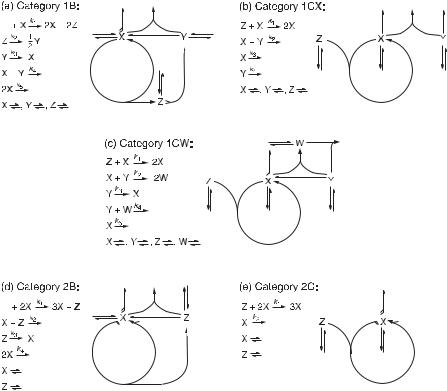
Fig. 11.4 Network diagrams and mechanisms for the prototypes of five categories: (a) category 1B; (b) category 1CX; (c) category 1CW; (d) category 2B; (e) category 2C. (Adapted from [9].)

oscillator and all the cycle species are type X species, the species taking part in the exit reaction are type Y species, and the species providing negative feedback is of type Z. A weak cycle cannot produce instability by adding an exit (or other) reaction. A refined fomulation of detailed conditions for the occurrence of the Hopf bifurcation is provided in [49].

Typically there is a cyclic pathway in oscillatory reaction networks, even though there exist cases when oscillatory instability is associated neither with a cycle in the network [50] nor with a positive feedback [38]. However, the following categorization assumes the presence of a cyclic pathway, since the vast majority of chemical oscillators possess this feature (future extensions are of course possible).

11.2.5 Categorization of Oscillatory Reactions

The categories of oscillators discussed in Eiswirth et al. [1] contain topologically different connectivity between the species, that is, the relations among the species in a system, as products and reactants in elementary mechanistic steps, which can produce

oscillatory behavior. Two main categories of oscillators are based on the autocatalytic cycle present in the mechanism. Category 1 is the group of oscillators with a critical cycle combined with an exit reaction; this implies that type Y species is always involved, in addition to type X and Z. Category 2 is a group of oscillators with strong cycles; here a direct removal of a cyclic species instead of an exit reaction is sufficient, and thus type Y is absent. Further classification of mechanisms leads to subcategories 1B, 1C (further subdivided into 1CX and 1CW) and 2B, 2C.

Figure 11.4a–e introduces prototypical examples of these categories. The figure provides elementary mechanistic steps for each prototype along with the corresponding network diagrams, each of them having distinctive topological features as described below.

Subcategories within this classification scheme are distinguished according to the kind of negative feedback involving type Z species:

1.Input negative feedback (Jzx Jxz < 0). Type Z species is flowed into the reactor and controls the autocatalytic process by reacting with the type X species; this

feature may occur in both category 1 (fig. 11.4b,c) and 2 (fig. 11.4e). Additionally, in category 1, type Z species may also be produced by an exit reaction (i.e., X + Y → Z) rather than provided via feed.

2.Output negative feedback (Jzx Jxy Jyz < 0). Type Z species is a product of a cycle reaction (such a reaction is termed tangent) and controls the autocatalysis indirectly by producing type Y species that inhibits the type X species (tangent feedback, see fig. 11.4a); in another variant of this kind of indirect control the type Z species is produced by exit rather than tangent reaction, and then produces type Y species (exit feedback). For category 2, the feedback expressed by JMEs is formally the same as for the input feedback, but Z is produced rather than consumed by an autocatalytic cycle reaction; in the next step Z reacts directly with X in an

exit reaction thereby leaving out type Y species. This represents tangent feedback (fig. 11.4d), but exit feedback may occur as well (e.g., via Z + X → 2Z).

The subcategories 1C (fig. 11.4b,c) and 2C (fig. 11.4e) involve mechanisms with input feedback; either Z or Y (or both) has to be provided by feed and thus the C subcategory is crucially dependent on inflow (C stands for continuous). The subcategories 1B (fig. 11.4a) and 2B (fig. 11.4d) involve mechanisms with output feedback, tangent or exit. Here the autocatalytic process is driven by a nonessential species (of type A or C) present in surplus and thus all essential species are generated by reactions rather than inflow. Consequently, reactions in the B subcategory provide sustained oscillations even in a closed system until the nonessential species is exhausted (B stands for batch). The 1C subcategory can be further divided into the subcategories 1CW (fig. 11.4c) and 1CX (fig. 11.4b). The former involves a new essential species of type W, which removes the type Y species and thus enables the autocatalysis to recover, whereas the latter accomplishes the same without the presence of W just by a slow inflow of X.

In category 1, the order of the autocatalytic species in the cycle reaction is equal to one (and equal to the order of X in the exit reaction). Category 2 oscillators include mechanisms with autocatalytic reaction of a higher (effective) order in X than the order of X in the removal reaction, and the type X species need not necessarily be chemical species. Rather, they may include vacant surface sites in heterogeneous catalysis, or temperature in thermokinetic oscillation.