

112 DETERMINATION OF COMPLEX REACTION MECHANISMS
also. The finding of the trend, that of negative feedback and reciprocal regulation, is important because it is the regulatory pattern expected from a simple, qualitative analysis of homeostasis, which is the task that the system is roughly expected to represent. In a physiological system, the concentration of a reservoir is affected by the fluxes into and out of the reservoir. A homeostatic mechanism should then seek to control these fluxes so that the concentration does not change, at least not significantly. For example, a mechanism to buffer the concentration of F should inhibit influx into F as the concentration of F rises (or potentiate efflux, or both), but do the opposite as the concentration of F drops. If the signal for these changes is F itself, and if the reaction structure of the pathway is the one we have modeled, we should expect that F inhibit β, the enzyme that produces its precursor, and potentiates α, which consumes its direct product. A similar action for T is likewise expected. While our model stops short of describing a homeostatic system, in that the reservoir concentrations are not affected by the behavior of the futile cycle, we may imagine reservoir concentrations being changed by the simultaneous action of a large number of identically regulated cycles. In that case, the regulatory pattern we find matches the one expected for homeostasis.
The class designations in table 10.1 refer to different types of switching regions where the concentrations of A and B exchange places due to the imposed variations of the reservoir concentrations. In classes A, B, C, and G this switching occurs rapidly, in classes E and F slowly, and in class D not at all. Networks of class D have eliminated one enzyme. But such gross features do not mark members of the other classes. In fact, for the other classes, the limiting network diagram is not sufficient to determine the class and thus the response behavior. This means that the specific regulatory parameters must be known in addition to the gross regulatory structure. It also means that a class of behavior may be realized by more than one regulatory structure. Further, members of a given class may show rather different performances. For example, class C is represented by networks I.3, III.3, and IV.4, which, however, have very different performances. Detailed knowledge of regulation is required even for qualitative predictions of performance. A final observation on the results in table 10.1 is that certain classes of behavior are more likely to appear on some courses than others. For instance, course I produced more members of class A than any other; in fact, only class C also appeared on that course. On the other hand, course V gave no members of classes A or C and gave more members of class E than B.
A comparison of performance on the several courses, made in more detail in [2] than presented here, shows that no single network does best on all five courses. There is no single winner as the environment represented by the courses changes, and thus no single species has global dominance. There are some specialists who do particularly well on one course, but of those not all survive the other courses. The winners are survivors that perform adequately from course to course, but not necessarily outstandingly; they differ from each other and thus present the opportunity for biological diversity.
10.3Evolutionary Development of Biochemical Oscillatory Reaction Mechanisms
We investigate in this section the application of genetic algorithms to the evolutionary development of a reaction mechanism. We choose as a particular example a part of
APPLICATIONS OF GENETIC ALGORITHMS |
113 |
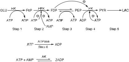
glycolysis modeled by the mechanism shown in fig. 10.3 [11]. This reaction can be in a single stable stationary state for given ranges of influx rates of glucose and adenylate pool concentrations (the sum of the concentrations of AMP, ADP, and ATP). However, for different ranges of these two quantities the reaction can be in an oscillatory state, a limit cycle, in which all the metabolite concentrations vary periodically; the variations in this highly nonlinear system are not sinusoidal. (For more on oscillatory reactions, see chapter 11.) Such oscillations have been observed in this reaction, in cell-free extracts of yeast cells, and in whole yeast cells themselves under anaerobic conditions.
Several purposes have been suggested for oscillatory reactions in biological systems. Oscillatory reactions tend to be more stable, and more resistant to external perturbations than comparable systems in a stationary state. The utilization and production of chemical species can be more efficient under oscillatory conditions. For example, in glycolysis with a given, constant input of glucose, the ratio of concentrations of ATP, the energyrich species, to ADP can be substantially increased in an oscillatory state compared to a stationary state. For an oscillatory input of glucose into an oscillatory reaction mechanism such as fig. 10.3 the ATP/ADP ratio changes; both increases and decreases can be effected with changes in the amplitude and frequency of the oscillatory glucose input. External periodic perturbations of such reactions in concentration, temperature, pressure, light intensity, or imposed electric fields can phase shift the oscillatory rate compared to the oscillatory Gibbs free energy change, with consequent changes in the dissipation and conversely in the efficiency of the reaction [12–16]. Similar phase shifts occur in alternating current (AC) networks, where the analog of the rate is the current, and that of the Gibbs free energy change is proportional to the voltage. These effects of an “AC chemistry” have been shown in experiments on the oscillatory horseradish peroxidase reaction by external periodic variation of the oxygen influx concentration into the system [17,18], in photosynthesis in a C3 plant [19,20], and in theoretical studies in proton transfer [15,21] and combustion reactions [22,23].
Our interest in this problem was kindled by a report on experiments that appeared in 1987 [24]; it showed that the impact of water waves in intertidal zones enhances
Fig. 10.3 A simple model of the reaction mechanism of glycolysis. For definition of symbols see fig. 6.1. FDP, fructose diphosphate; PYR, pyruvate; LAC, lactate. (From [11].)

114 DETERMINATION OF COMPLEX REACTION MECHANISMS
Table 10.2 Values of the enzymatic binding constants at autonomous oscillations for constant influx of glucose
|
|
A |
B |
C |
D |
E |
|
|
|
|
|
|
|
Parameter |
Experimental value |
GA (one variable) |
pmax |
GA (two variable) |
pmax |
|
α1 |
= kRAMP/K2ATP,T |
0.417 |
0.25–0.45 |
0.8 |
0.25–0.45 |
0.8 |
α2 |
= KRFru-1,6-P2 /K4ATP,T |
0.0215 |
0.075 |
— |
0.053–0.954 |
0.8 |
Adenylate pool |
40.95 |
41.3 |
|
41.3 |
|
|
|
concentration (mM) |
|
|
|
|
|
|
|
|
|
|
|
|
The values of enzymatic binding constants at autonomous oscillations for constant influx of glucose are given in column A. We define two ratios of binding constants as variables: α1 = KRAMP /K2ATP,T for the second reaction (step 2) in fig. 10.3, and
α2 = KRFru-1,6-P2 /K4ATP,T for the fourth reaction (step 4). Variable ranges in the GA are given for one-variable and two-variable cases. The maximum change of the parameter pmax (see text) is determined in such a way that the middle values of variables are in the vicinity of the bifurcation. At the initial values of α1 and α2 for both one-variable and two-variable GA cases, this model has a single stationary state. We set the adenylate pool concentration to be 41.3 mM for our study. (From [11].)
the biological growth of intertidal organisms. The authors offer four possible reasons:
(1)“waves aid in protecting intertidal inhabitants from their principal enemies”;
(2)“waves strip away the boundary layer of used water from kelp blades, thus facilitating nutrient uptake”; (3) “waves apparently enhance algal productivity by allowing algae to use light more efficiently”; and (4) “waves enable some of the shore’s more productive inhabitants to displace their competitors.” Furthermore, they add, “in general, intertidal zones of the northeastern Pacific are more completely covered by plants and animals the more exposed they are to wave action.”
We search for an additional reason, one based on the possibility that oscillatory reactions in biological systems may have developed in evolution in response to periodic perturbations of water waves impacting on rocks at the shore of a sea. For this purpose we use the model reaction mechanism in fig. 10.3. Oscillations in this system may occur and these are due to the presence of feedback and feedforward loops, such as the binding of ATP and ADP to the enzymes PFK and PK, and the binding of FDP to PK. We want to change these binding constants so that no oscillations occur and take that system as our starting point. We abbreviate enzymatic binding and rate coefficients by EBR, and
consider four dissociation constants for ligands bound to the R and T conformations (KRAMP, K2ATP,T , KRAMP, K4ATP,T ) for phosphofructokinase (PFKase) and pyruvate kinase
(PKase), respectively, and in turn we define two ratios α1 = KRAMP/K2ATP,T and α2 = KRFru-1,6-P2 /K4ATP,T as variables. The values of these variables for which autonomous oscillations occur at constant influx of glucose are given in table 10.2; for details on rate coefficients, see [25].
We start the GA procedure by choosing an influx of glucose and the adenylate pool concentration (the sum of the concentrations of AMP, ADP, and ATP) such that this reaction mechanism has a single stable stationary state; in table 10.2, the initial value of α1 used in the GA is the first number given in the second column and the initial value of α2 is the first number in the fourth column. We then compare the evolutionary development of two types of such systems, one with a constant influx of glucose and
APPLICATIONS OF GENETIC ALGORITHMS |
115 |
the other with an oscillatory influx of glucose, to model the periodic effect of waves impinging on an organism. We allow a given initial choice of the EBR to vary by small random increments from one generation to the next, first for one variable and then for two, and carry out this variation systematically by means of a numerical GA method. For our study, we wish to optimize the ratio ATP/ADP, and assume that this ratio is a correlative measure of the rate of growth of an organism. The questions to be asked then are:
1.What is the relative development in time with the GA-controlled variation of the EBR of the two types of systems, one with constant influx of glucose, the other with an oscillatory influx of glucose, with average influx the same as in the constant influx case?
2.How will the ATP/ADP ratio produced by the GA variation of the EBR compare in the two types of systems?
3.What are the changes as we go from one to two variables?
4.What bearings do the answers to these questions have on the issue of the evolutionary development of oscillatory biological reactions and the experimental observations [24]?
The GA works by encoding a parameter of the EBR into a binary string. The algorithm evolves parameter sets by the operations of selection, crossover, and mutations into the strings from one generation to the next. A variable p has a simple form, pin ·(1+pmax ·R/ (216 − 1)), where pin is the initial value of p, pmax gives the maximum change of the parameter not per generation but overall, and R is initially set to be zero; then a binary string corresponding to R is evolved within the range 0 ≤ R ≤ 216 − 1 by the GA operations. In the GA, we assign strings for 24 individuals for the variables in the EBR, searching for the change from the initial stable stationary state to autonomous oscillation. We set the maximum change of each variable per generation within ±7%.
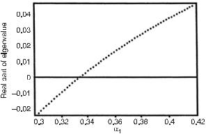
We begin with the genetic algorithm variation of one variable and choose for that the parameter α1. Further, we choose the adenylate pool to be constant at 41.3 mM; α2 is set to be constant at 0.075. The stationary states of the kinetic equations for this system (see [13]) yield the bifurcation diagram shown in fig. 10.4, which is a plot of
Fig. 10.4 Bifurcation diagram for the adenylate pool at 41.3 mM with α2 = 0.075. The real part of the temporal eigenvalues of the linearized kinetic equations is plotted versus the parameter α1. The bifurcation occurs after α1 = 0.334. (From [11].)
116 DETERMINATION OF COMPLEX REACTION MECHANISMS
the real part of the temporal eigenvalues of the linearized kinetic equations versus the parameter α1. For α1 < 0.334, the real part is negative, and the stationary state is either a stable focus or a node. For α1 > 0.334, the stationary states are unstable foci and evolve to a stable limit cycle with a period of 0.505 min in the vicinity of the bifurcation. In the application of the GA we compare two different systems; one has a constant influx of glucose (the flow, Vconst = 2 mM/min) and the other has a sinusoidal oscillatory influx of glucose with the same average flux as that of the constant influx, that is, Vosc = Vconst + a sin[(2π T )t], where a is the amplitude and T is the period of the oscillation. For each of the two types of systems, we select 24 copies (individuals), each with an initial value of the parameter α1 = 0.25, such that no oscillations occur. We set pmax to be 0.8, such that the middle value of α1 (0.35) (see table 10.2) is in the vicinity of the bifurcation. In each new generation, the binary strings of α1 are evolved by the GA operators within a range such that the new highest value of the parameter in any one generation does not differ by more than 7% from the prior generation. The kinetic equations (see eqs. 1–16 and 21 in [25]) are then solved for each of the 24 individuals and from these solutions we record the state attained for each individual, either stationary or oscillatory. We define the ratio of ATP/ADP in units of its initial value. For the stationary case, the ratio is (ATP/ADP)stat /(ATP/ADP)α1 =0.25, where (ATP/ADP)stat is the ratio of ATP/ADP in a stationary state and(ATP/ADP)α1 =0.25 is the ratio of the initial stationary state at α1 = 0.25. For the oscillatory case, the ratio is (ATP/ADP)osc(ATP/ADP)α1 =0.25, where (ATP/ADP)osc is time averaged over one period of the oscillation. In each generation and in each group of 24, we select the system with the highest ATP/ADP ratio and pass that individual to the next generation; we change the worst performer to equal the best performer, and we alter the remaining individuals by mutations and recombinations prior to passing them on to the next generation. As the number of generations increases, the individuals attain higher values of the parameter α1 up to and beyond the bifurcation.
In the oscillatory influx of glucose, we drive the initially stable focus with a given period (frequency) and amplitude of the imposed sinusoidal glucose oscillation (a = 0.5 mM/min). Before the bifurcation, the system is either in a stable node or stable focus and responds to the imposed periodic influx of glucose with the same period as that of the influx. After the bifurcation, the period of the response may differ from the period of the autonomous oscillation. Considering the period as a parameter, we observe that if this period is less than the period of the autonomous oscillation (0.5 min) in the vicinity of the bifurcation, the value of the ATP/ADP ratio can be maximized before the bifurcation; for instance, if the driving period is set to be 0.43 min, the value of the ATP/ADP ratio is (locally) maximized before the bifurcation. After the bifurcation, the value of the ATP/ADP ratio decreases with the fixed external period. This decrease is caused by the existence of a narrow entrainment band of the frequency in response to the external oscillatory influx. However, if the fixed external period after the bifurcation is outside the entrainment band [26], then the value of the ATP/ADP ratio is decreased.
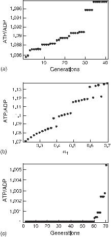
The result for the one-variable case is shown in fig. 10.5(a) for an oscillatory influx of glucose. The point at the 30th generation is at the bifurcation. In fig. 10.5(b), the ATP/ADP ratio as a function of α1 (deterministic) is plotted, and the plot shows bistable behavior after the bifurcation (α1 > 0.334). Note the increase in the ATP/ADP ratio. An analogous plot for a constant input of glucose is given in fig. 10.5(c), in which the
APPLICATIONS OF GENETIC ALGORITHMS |
117 |
Fig. 10.5 Plot of the ATP/ADP ratio versus
(a) the number of generations in the GA,
(b) α1 for the oscillatory influx of glucose with the amplitude 0.5 mM/min (deterministic case),
(c) the number of generations for the constant influx of glucose. In (a) and (c), the highest value of the ATP/ADP ratio among 24 individuals at each generation by the GA is plotted and shows that systems with the constant influx of glucose take about double the generations necessary to reach the autonomous oscillation than systems with the oscillatory influx of glucose. (From [11].)
bifurcation is reached at the 60th generation; the value of the ATP/ADP ratio does not change before the bifurcation and only a very small increase in the ATP/ADP ratio occurs just at the bifurcation.
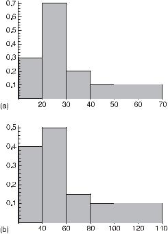
The kinetic equations we solve are deterministic, but stochastic (probabilistic) elements are introduced in the GA. Hence, individuals in a given group arrive at the bifurcation after different numbers of generations. Thus, we generate a frequency distribution for the arrival at the bifurcation as a function of the generation number. This frequency density for an individual reaching the bifurcation differs for the oscillatory input (fig. 10.6a) compared to the constant input of glucose (fig. 10.6b). The most probable value of the generation reaching the bifurcation is 30 for the oscillatory input and substantially larger, 59, for the constant input.The results for the genetic algorithm variation of two variables are similar and are included in the following summary of this study.
The imposition of an oscillatory influx of glucose on the reaction mechanism shown in fig. 10.3, initially in a state of no oscillations (in a node or a focus), may have
118 DETERMINATION OF COMPLEX REACTION MECHANISMS
Fig. 10.6 The frequency density versus number of generations to reach the bifurcation: (a) the oscillatory influx (average 30) and (b) the constant influx (average 59). (From [11].)
two evolutionary advantages over the same system with a constant influx of glucose: (1) as shown for the example discussed, a higher ATP/ADP ratio is reached at the bifurcation; and (2) the bifurcation is reached more quickly. For the case of the variation of a single variable with a constant influx of glucose, it takes, for the most probable development, 59 generations to reach oscillatory conditions with increased ATP/ADP ratio of 1.0004. For oscillatory input, this number is reduced to 30 generations with higher ATP/ADP ratio of 1.1. In the variation of two variables, for the constant input case, the number of generations necessary to reach the autonomous oscillation is 167 generations with increased ATP/ADP ratio of 1.0004 and, for the oscillatory glucose input, 76 generations with a higher ATP/ADP ratio of 1.1. We see that the more variables are evolved, the more generations are necessary to reach autonomous oscillations—about tripled (from 59 to 167) for the constant input case and more than doubled (from 30 to 76) for the oscillatory glucose input. These results are obtained from the deterministic kinetic calculation and, with the application of the GA, show the driving force toward the bifurcation.
Both advantages suggest that the evolutionary development of oscillatory reactions, at least in glycolysis, may have occurred at rocks on shores because of the periodic impact of water waves. The faster development of oscillations with periodic wave impact (differences of time scales of many mutations) ensures the spread of that development away from those shores. The individuals subjected to wave impacts have a higher ATP/ADP ratio than those in tidal inlets without such wave impacts, and growth at the shore may therefore expected to be higher, as found by observations [24].

APPLICATIONS OF GENETIC ALGORITHMS |
119 |
10.4Systematic Determination of Reaction Mechanism and Rate Coefficients
In this section we illustrate the use of genetic algorithms for the determination of reactions mechanisms and rate coefficients from measurements [27]. We apply the optimization method to the cerium catalyzed minimal bromate system, which has been investigated in some detail. This nonlinear system, when open to mass flow, can be in a single stationary state, a node or a focus, or an unstable focus that suggests a stable limit cycle. The return of a system to a stable node, near that node, is given by an exponential decay with a real rate coefficient; the return to a stable focus is given by an exponential decay with a complex rate coefficient that has a negative real part; in that case the system returns to the stable focus with damped oscillations in concentrations. We take it as given, that is, as determined by experiments, that the chemical species in this system are
BrO−3 , HBrO2, HOBr, BrO•2, Br−, H+, Ce4+, Ce3+, Br2, H2O (10.9)
This reaction has been modeled by several mechanisms; one is the NFT mechanism [28,29], which is an important part of the FKN (Field–Körös–Noyes) mechanism [30] of the oscillatory Belousov–Zhabotinsky reaction [31,32]. Its complex behavior has been studied experimentally in a continuous-flow stirred tank reactor (CSTR) [33]. The rate equations for such an open system are described in a vector form by
dC
(10.10)
dt
where f(C) is the mass action rates of individual reactions; C is a concentration vector
for the species; v is a stoichiometric matrix of the species; C0 is a feed (BrO3−, Br−, H+, |
||||||||||||||||||
Ce+) concentration vector; and k |
0 |
(C |
− |
C |
0 |
) describes the flow terms with flow rate k |
0 |
. |
||||||||||
3 |
|
|
|
|
|
|
|
|
|
|
|
|
|
|
||||
In steady states, there are element balance conditions for the reactions [34]: |
|
|
|
|||||||||||||||
|
|
|
|
|
|
A · δn = 0 |
|
|
|
|
|
(10.11) |
||||||
where the system formula matrix (or atomic matrix) A is given by |
|
|
|
|||||||||||||||
A |
3 |
2 |
1 |
|
2 |
|
0 |
0 |
0 |
0 |
0 |
1 |
(10.12) |
|||||
|
|
1 |
1 |
1 |
|
1 |
|
1 |
0 |
0 |
2 |
0 |
0 |
|
|
|
|
|
|
= 0 0 0 |
|
0 |
|
0 |
0 |
1 |
0 |
1 |
0 |
|
|
|
|||||
|
|
0 |
1 |
1 |
|
0 |
|
0 |
1 |
0 |
0 |
0 |
2 |
|
|
|
|
|
|
|
|
|
|
|
|
|
|
|
|
|
|
|
|
|
|
|
|
and the element balance vector δn is |
|
|
|
|
|
|
|
|
|
|
|
|
|
|||||
δn = δBrO3− , δHBrO2 , δHOBr , δBrO2• , δBr− , δH+ , δCe4+ , δBr2 , δCe3+ , δH2 O |
(10.13) |
|||||||||||||||||
The set of null-space vectors of the matrix A represents the independent reactions that satisfy the stoichiometric condition of mass conservation. If we select all possible bimolecular reactions among all the species, but permit H2O and H+ to be additional reactants, and impose conservation of atoms and charge, then we find that linear combinations of the independent reactions yield seven elementary steps:
1.Br− + BrO−3 + 2H+ HBrO2 + HOBr
2.Br− + HBrO2 + H+ 2HOBr
3.Br− + H+ + HOBr Br2 + H2O
4.BrO−3 + H+ + HBrO2 2BrO•2 + H2O
120 DETERMINATION OF COMPLEX REACTION MECHANISMS |
|
||
5. |
Ce3+ + BrO2• |
+ H+ Ce4+ + HBrO2 |
|
6. |
Ce4+ + BrO2• |
+ H2O BrO3− + Ce3+ + 2H+ |
|
7. |
2HBrO2 BrO3− + H+ + HOBr |
(10.14) |
|
which constitute precisely the NFT mechanism. This result is accidental; for example, it is not the result in the Citri–Epstein mechanism for the chlorite–iodide reaction [35]. In the literature [30] the NFT mechanism is represented by the following overall reaction:
BrO3− + 4Ce3+ + 5H+ 4Ce4+ + HOBr + 2H2O |
(10.15) |
We now check the consistency between the overall reaction (eq. (10.15)) and the elementary steps (eq. (10.14)), we need to find out how many of each of the elementary steps (eq. (10.14)) are necessary for the generation of the overall reaction. We designate the stoichiometric vector attached to the overall reaction (eq. (10.15)) as
noverall = (−1, 0, 1, 0, 0, −5, 4, 0, −4, 2) |
(10.16) |
where the negative sign is for a reactant and the positive for a product; see the order of species in eq. (10.13). From the overall reaction (eq. (10.15)) we see that there are four intermediate species, Br−, HBrO2, BrO•2, Br2. To obtain the overall reaction, we add up the elementary steps, each of the elementary reactions being multiplied by a stoichiometric number [36]. In the result, we require that the stoichiometric coefficients of the intermediates be equal to zero. In other words, the total number of ith intermediates created by all S steps, fi , must vanish, that is,
S |
|
|
|
fi = bis ns = 0 |
(10.17) |
s=1
where ns is the stoichiometric number for the sth reaction step, and bis is the stoichiometric coefficient of ith intermediates in the sth step. Equations (10.17) express the condition that in the overall reactions the stoichiometric coefficients of the active intermediates are equal to zero. Therefore, the null-space of the matrix B represents the overall reactions. To satisfy the overall reaction (eq. (10.15)), there must be included at least one of the following vector sets of elementary reaction steps in the NFT mechanism, (eq. (10.14)):
v == {(4, 5, 7), (4, 6, 7), (5, 6, 7), (1, 2, 4, 5), (1, 2, 4, 6), (1, 2, 5, 6)} |
(10.18) |
Consider the set v1 = (4, 5, 7) as an example, where the matrix B is given by the stoichiometric coefficients of the intermediates Br−, HBrO2, BrO•2, Br2 in the steps (4,5,7);
B(v1) |
−2 |
−1 |
0 |
(10.19) |
||
|
= |
1 |
1 |
2 |
|
|
|
0 |
0 |
0 |
|
||
|
|
0 |
0 |
0 |
|
|
|
|
|
|
|
|
|
Then, the null space of B(v1) yields a stoichiometric number vector nv1 = (−2, −4, 1) and the overall reaction (eq. (10.15)) is nv1 ‚ v1. As a result, there are 3 three-step, 13 four-step, 16 five-step, and 7 six-step combinations that satisfy this requirement. We apply GAs to search for oscillatory reaction mechanisms among those sets of reactions.
In the search for an oscillatory reaction mechanism we use as optimization criterion available experimental results. Bar-Eli and Geiseler [28] carried out experiments to
APPLICATIONS OF GENETIC ALGORITHMS |
121 |
determine the domain of oscillations in the subspace of a range of the initial bromide and bromate concentrations at fixed inflow concentrations of cerium ion and acid. The extent of this experimental domain is estimated from their results given in fig. 3 of [28]. To complicate matters, there are unfortunately several sets of rate coefficients that have been obtained from a variety of investigations; there is reasonable agreement among these sets for some of the rate coefficients and substantial disagreement among others (by several orders of magnitude).
The first GA search was for oscillations in the possible reaction mechanisms given that the GA may vary the influx bromide and bromate concentrations over ranges that include the observations in [28]. For that purpose we used the so-called NFT rate coefficients. Under these conditions, no oscillations were found in any of the three possible three-step mechanisms. The GA reveals that there are two different groups of oscillatory mechanisms in the four-step and five-step sets. The first group of reaction sets of elementary steps consists of the reactions (1,2,4,5), (1,2,4,5,6), and (1,2,4,5,7). For this group, the form of the oscillations is shifted only in phase among these three reaction mechanisms; thus, the four-step (1,2,4,5) is an irreducible mechanism and the elementary steps 6 or 7 are not essential for an oscillatory mechanism.
The second group consists of reactions (1,2,3,4,5) and (1,2,3,4,5,6,7). The two sets involve ten species of which five are independent species. The forms of the oscillations in these two sets are identical; therefore, the five-step (1,2,3,4,5) is an irreducible set and steps 6 and 7 are (again) not essential steps in the seven NFT steps with the FKN rate coefficients. In the mechanisms of both groups I and II, there are five essential species, HBrO2, HOBr, BrO•2, Br−, Ce+3 , which are necessary to have oscillations in the NFT mechanism. Although the above oscillatory domains are near the experimental one, and the periods and shapes of the oscillations are compatible with the experimental results, both group I and II reaction mechanisms with the FKN rate coefficients do not fit experimental results well.
Next, we focus on the fourand five-step mechanisms in groups I and II. We do a GA search for optimal rate coefficients that yield unstable foci at four experimental points in the bromide–bromate concentration plane, and find excellent agreements with the experiments.
The GA reveals that the four-step (1,2,4,5) mechanism exhibits oscillations, but not in the experimental domain. On the other hand, for the five-step mechanism (1,2,3,4,5), the GA finds rate coefficients that give very good agreement with all comparable experiments. The period of waves generated by the five-step mechanism is in excellent agreement with the experiments. The shape of waves is very similar to the experimental waves, but a quantitative comparison of the calculated waves with the experimental was not attempted. Although the four-step mechanism displays oscillation, it fails to reproduce the experimental oscillation domain. The five-step mechanism, which is made up of the four steps in the four-step mechanism plus the additional reaction step 3, manages to reproduce the experimental domain. It follows that the reaction step 3 is essential for agreement with the experiments.
With the use of the five forward rate coefficients found by the GA that yield unstable foci for all four experimental condition, we search again which ones of the possible three, four, and five steps have oscillation domains comparable to the experiments. The GA shows that no reaction mechanism other than those of groups I and II have oscillations in the experimental range. Thus, the oscillatory five-step mechanism consisting of the