

B.Crowell - Electricity and Magnetism, Vol
.4.pdf5.5Two or Three Dimensions
(a) A 19th century USGS topographical map of Shelburne Falls, Mass.
3V
2V
1V
(b) The constant-voltage curves surrounding a point charge. Near the charge, the curves are so closely spaced that they blend together on this drawing due to the finite width with which they were drawn. Some electric fields are shown as arrows.
The topographical map shown in figure (a) suggests a good way to visualize the relationship between field and voltage in two dimensions. Each contour on the map is a line of constant height; some of these are labeled with their elevations in units of feet. Height is related to gravitational potential energy, so in a gravitational analogy, we can think of height as representing voltage. Where the contour lines are far apart, as in the town, the slope is gentle. Lines close together indicate a steep slope.
If we walk along a straight line, say straight east from the town, then height (voltage) is a function of the east-west coordinate x. Using the usual mathematical definition of the slope, and writing V for the height in order to remind us of the electrical analogy, the slope along such a line is V/ x, or dV/dx if the slope isn’t constant.
What if everything isn’t confined to a straight line? Water flows downhill. Notice how the streams on the map cut perpendicularly through the lines of constant height.
It is possible to map voltages in the same way, as shown in figure (b). The electric field is strongest where the constant-voltage curves are closest together, and the electric field vectors always point perpendicular to the constant-voltage curves.
The figures on the following page show some examples of ways to visualize field and voltage patterns.
Mathematically, the calculus of the preceding section generalizes to three dimensions as follows:
Ex = –dV/dx
Ey = –dV/dy
Ez = –dV/dz
Self-Check
Imagine that the topographical map represents voltage rather than height.
(a) Consider the stream the starts near the center of the map. Determine the positive and negative signs of dV/dx and dV/dy, and relate these to the direction of the force that is pushing the current forward against the resistance of friction. (b) If you wanted to find a lot of electric charge on this map, where would you look?
(a) The voltage (height) increases as you move to the east or north. If we let the positive x direction be east, and choose positive y to be north, then dV/dx and dV/dy are both positive. This means that Ex and Ey are both negative, which makes sense, since the water is flowing in the negative x and y directions (south and west). (b) The electric fields are all pointing away from the higher ground. If this was an electrical map, there would have to be a large concentration of charge all along the top of the ridge, and especially at the mountain peak near the south end.
Section 5.4ò Voltage for Nonuniform Electric Fields |
121 |
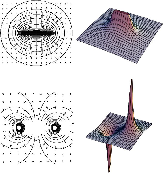


 –
–


 +
+ 


Two-dimensional field and voltage patterns.
Top: A uniformly charged rod. Bottom: A dipole.
In each case, the diagram on the left shows the field vectors and constant-voltage curves, while the one on the right shows the voltage (up-down coordinate) as a function of x and y.
Interpreting the field diagrams: Each arrow represents the field at the point where its tail has been positioned. For clarity, some of the arrows in regions of very strong field strength are not shown — they would be too long to show.
Interpreting the constant-voltage curves: In regions of very strong fields, the curves are not shown because they would merge together to make solid black regions.
Interpreting the perspective plots: Keep in mind that even though we’re visualizing things in three dimensions, these are really two-dimensional voltage patterns being represented. The third (up-down) dimension represents voltage, not position.
122
5.6*ò Electric Field of a Continuous Charge Distribution
L
Charge really comes in discrete chunks, but often it is mathematically convenient to treat a set of charges as if they were like a continuous fluid spread throughout a region of space. For example, a charged metal ball will have charge spread nearly uniformly all over its surface, and in for most purposes it will make sense to ignore the fact that this uniformity is broken at the atomic level. The electric field made by such a continuous charge distribution is the sum of the fields created by every part of it. If we let the “parts” become infinitesimally small, we have a sum of an infinite number of infinitesimal numbers, which is an integral. If it was a discrete sum, we would have a total electric field in the x direction that was the sum of all the x components of the individual fields, and similarly we’d have sums for the y and z components. In the continuous case, we have three integrals.
|
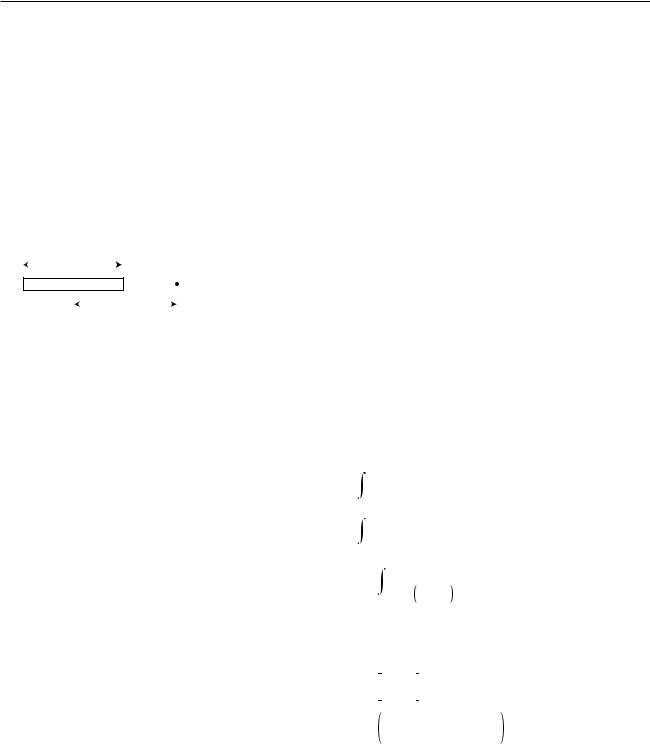
Example: field of a uniformly charged rod |
|
Question: A rod of length L has charge Q spread uniformly along |
|
it. Find the electric field at a point a distance d from the center of |
|
the rod, along the rod’s axis. |
|
Solution: |
d |
Let x=0 be the center of the rod, and let the positive x axis be |
|
to the right. This is a one-dimensional situation, so we really only |
|
need to do a single integral representing the total field along the |
|
x axis. We imagine breaking the rod down into short pieces of |
|
length dx, each with charge dq. Since charge is uniformly spread |
|
along the rod, we have dq=(dx/L)Q. Since the pieces are infini- |
|
tesimally short, we can treat them as point charges and use the |
|
expression kdq/r2 for their contributions to the field, where r=d–x |
|
is the distance from the charge at x to the point in which we are |
|
interested. |
Ex |
= |
|
k dq |
|
|||
|
|
r 2 |
|
|
|||
|
= |
L / 2 |
k dx Q |
||||
|
L / 2 |
|
L r 2 |
||||
|
|
|
|||||
|
= |
kQ |
|
L / 2 |
dx |
||
|
L |
– L / 2 |
d – x 2 |
||||
|
|
||||||
The integral can be looked up in a table, or reduced to an elementary form by substituting a new variable for d-x. The result is
Ex |
= |
kQ |
|
1 |
|
|
L / 2 |
||||
|
|
||||||||||
|
|
|
|
|
|
|
|||||
L |
|
d – x |
|
|
– L / 2 |
||||||
|
|
|
|
|
|||||||
|
|
kQ |
1 |
1 |
|
||||||
|
= |
L |
|
– |
|
. |
|||||
|
d – L / 2 |
d + L / 2 |
|||||||||
For large values of d, the expression in brackets gets smaller for two reasons: (1) the denominators of the fractions become large, and (2) the two fractions become nearly the same, and tend to cancel out. This makes sense, since the field should get weaker for larger values of d.
It is also interesting to note that the field becomes infinite at the ends of the rod, but is not infinite on the interior of the rod. Can you explain physically why this happens?
Section 5.5*ò Electric Field of a Continuous Charge Distribution |
123 |

Summary
Selected Vocabulary |
|
field ........................................ |
a property of a point in space describing the forces that would be |
|
exerted on a particle if it was there |
sink ........................................ |
a point at which field vectors converge |
source ..................................... |
a point from which field vectors diverge; often used more inclusively |
|
to refer to points of either convergence or divergence |
electric field ............................ |
the force per unit charge exerted on a test charge at a given point in |
|
space |
gravitational field.................... |
the force per unit mass exerted on a test mass at a given point in |
|
space |
electric dipole ......................... |
an object that has an imbalance between positive charge on one side |
|
and negative charge on the other; an object that will experience a |
|
torque in an electric field |
Notation |
|
g ........................................ |
the gravitational field |
E ....................................... |
the electric field |
D ....................................... |
an electric dipole moment |
Notation Used in Other Books |
|
d,p,m ................................. |
other notations for the electric dipole moment |
Summary
Newton conceived of a universe where forces reached across space instantaneously, but we now know that there is a delay in time before a change in the configuration of mass and charge in one corner of the universe will make itself felt as a change in the forces experienced far away. We imagine the outward spread of such a change as a ripple in an invisible universe-filling field of force.
We define the gravitational field at a given point as the force per unit mass exerted on objects inserted at that point, and likewise the electric field is defined as the force per unit charge. These fields are vectors, and the fields generated by multiple sources add according to the rules of vector addition.
When the electric field is constant, the voltage difference between two points lying on a line parallel to the field is related to the field by the equation V = –Ed, where d is the distance between the two points.
124 |
Chapter 5 Fields of Force |
Homework Problems
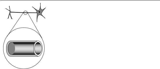
Problem 1.
1 . In our by-now-familiar neuron, the voltage difference between the
inner and outer surfaces of the cell membrane is about Vout-Vin = –70 mV in the resting state, and the thickness of the membrane is about 6.0 nm
(i.e. only about a hundred atoms thick). What is the electric field inside the membrane?
2. (a ) The gap between the electrodes in an automobile engine's spark plug is 0.060 cm. To produce an electric spark in a gasoline-air mixture, an electric field of 3.0x10⁶ V/m must be achieved. On starting a car, what minimum voltage must be supplied by the ignition circuit? Assume the field is constant. (b) The small size of the gap between the electrodes is inconvenient because it can get blocked easily, and special tools are needed to measure it. Why don’t they design spark plugs with a wider gap?
3. (a) At time t=0, a small, positively charged object is placed, at rest, in a uniform electric field of magnitude E. Write an equation giving its speed, v, in terms of t, E, and its mass and charge m and q.
(b) If this is done with two different objects and they are observed to have the same motion, what can you conclude about their masses and charges? (For instance, when radioactivity was discovered, it was found that one form of it had the same motion as an electron in this type of experiment.)
4↔. Show that the magnitude of the electric field produced by a simple two-charge dipole, at a distant point along the dipole’s axis, is to a good approximation proportional to D/r3, where r is the distance from the
dipole. [Hint: Use the approximation  1 + e
1 + e p » 1 +pe , which is valid for small e.]
5ò. Given that the field of a dipole is proportional to D/r3 (see previous problem), show that its voltage varies as D/r2. (Ignore positive and negative signs and numerical constants of proportionality.)
6ò. A carbon dioxide molecule is structured like O-C-O, with all three atoms along a line. The oxygen atoms grab a little bit of extra negative charge, leaving the carbon positive. The molecule’s symmetry, however, means that it has no overall dipole moment, unlike a V-shaped water molecule, for instance. Whereas the voltage of a dipole of magnitude D is proportional to D/r2 (see previous problem), it turns out that the voltage of a carbon dioxide molecule along its axis equals k/r3, where r is the distance from the molecule and k is a constant. What would be the electric field of a carbon dioxide molecule at a distance r?
7 ò. A proton is in a region in which the electric field is given by E=a+bx3. If the proton starts at rest at x1=0, find its speed, v, when it reaches position x2. Give your answer in terms of a, b, x2, and e and m, the charge and mass of the proton.
S |
A solution is given in the back of the book. |
↔ A difficult problem. |
|
A computerized answer check is available. |
ò A problem that requires calculus. |
Homework Problems |
125 |
8↔. Consider the electric field created by a uniform ring of total charge q and radius b. (a) Show that the field at a point on the ring’s axis at a distance a from the plane of the ring is kqa(a2+b2) –3/2. (b) Show that this expression has the right behavior for a=0 and for a much greater than b.
9òS.Consider the electric field created by an infinite uniformly charged plane. Starting from the result of problem 8, show that the field at any point is 2pks, where s is the density of charge on the plane, in units of coulombs per square meter. Note that the result is independent of the distance from the plane. [Hint: Slice the plane into infinitesimal concentric rings, centered at the point in the plane closest to the point at which the field is being evaluated. Integrate the rings’ contributions to the field at this point to find the total field.]
10ò. Consider the electric field created by a uniformly charged cylinder which extends to infinity in one direction. (a) Starting from the result of problem 8, show that the field at the center of the cylinder’s mouth is 2pks, where s is the density of charge on the cylinder, in units of coulombs per square meter. [Hint: You can use a method similar to the one in problem 8.] (b) This expression is independent of the radius of the
q1 cylinder. Explain why this should be so. For example, what would happen if you doubled the cylinder’s radius?
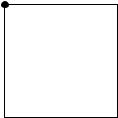
11 S. Three charges are arranged on a square as shown. All three charges  q2 are positive. What value of q2/q1 will produce zero electric field at the
center of the square?
q1 
Problem 11.
126 |
Chapter 5 Fields of Force |
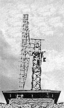
A World Ward II radar installation in
Sitka, Alaska.
6 Electromagnetism
Everyone knows the story of how the nuclear bomb influenced the end of World War II. The Hiroshima and Nagasaki bombings, however, came when Germany was already defeated and Japan’s surrender was only a matter of time.* Far less well known, but more important to the outcome of the war, was a different contribution from physics: radar. This new technology, based on the work of theoretical physicists James Clerk Maxwell in the previous century, played a decisive role in the air war known as the Battle of Britain. If not for the English radar defenses, Hitler might have succeeded in conquering Britain and gone on to win the war.
In this chapter, we discuss the magnetic field, its intimate relationship to the electric field, and the existence of waves made of electric and magnetic fields linked to each other.
*The bombings were a sad appearance of physics on the stage of history. Many of the physicists working on the bombs had assumed that they would only be used for demonstrations, not in a first strike on cities, but criticism after the fact was muted, partly because of relief that there would not have to be an invasion of Japan against fierce resistance. (On a personal note, both my grandfathers were in the Pacific during the war, and it’s not unlikely that they would have been killed during such an invasion.) Numerically, the number of people killed in the American firebombing of Tokyo was comparable to the number who died in the later nuclear attacks, and both were dwarfed by the toll of Chinese civilians raped or killed by the Japanese at Nanking, an atrocity that some have compared to the Holocaust. Nevertheless, one can’t help feeling that unleashing nuclear weapons for the first time was a different thing, a breaking of a kind of taboo. Many physicists, even those born after 1945, feel a sense of collective guilt that their art led to an era in which nuclear weapons endanger our whole biosphere. That era did not end along with the Cold War, and only time will tell whether nuclear weapons will be used again — in Pakistan and India, or somewhere else.
127
6.1 |
The Magnetic Field |
||
|
|
|
No magnetic monopoles |
|
|
S |
If you could play with a handful of electric dipoles and a handful of bar |
|
|
magnets, they would appear very similar. For instance, a pair of bar magnets |
|
|
S |
||
|
N |
||
|
wants to align themselves head-to-tail, and a pair of electric dipoles does the |
||
|
|
||
|
|
|
|
|
|
|
same thing. (It is unfortunately not that easy to make a permanent electric |
|
N |
S |
dipole that can be handled like this, since the charge tends to leak.) |
|
You would eventually notice an important difference between the two |
||
(a) |
|
N |
|
|
|
types of objects, however. The electric dipoles can be broken apart to form |
|
|
|
|
|
|
|
|
isolated positive charges and negative charges. The two-ended device can be |
|
|
|
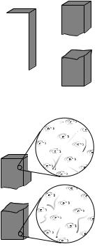
broken into parts that are not two-ended. But if you break a bar magnet in |
|
|
|
half, (a), you will find that you have simply made two smaller two-ended |
|
|
|
objects. |
|
|
|
The reason for this behavior is not hard to divine from our microscopic |
|
S |
|
picture of permanent iron magnets. An electric dipole has extra positive |
|
N |
|
“stuff” concentrated in one end and extra negative in the other. The bar |
|
|
|
magnet, on the other hand, gets its magnetic properties not from an |
|
|
|
imbalance of magnetic “stuff” at the two ends but from the orientation of |
|
S |
|
the rotation of its electrons. One end is the one from which we could look |
|
|
down the axis and see the electrons rotating clockwise, and the other is the |
|
|
N |
|
|
(b) |
|
one from which they would appear to go counterclockwise. There is no |
|
|
|
||
|
|
difference between the “stuff” in one end of the magnet and the other, (b). |
|
|
|
|
|
|
|
|
Nobody has ever succeeded in isolating a single magnetic pole. In |
|
|
|
technical language, we say that magnetic monopoles do not seem to exist. |
|
|
|
Electric monopoles do exist — that’s what charges are. |
Electric and magnetic forces seem similar in many ways. Both act at a distance, both can be either attractive or repulsive, and both are intimately related to the property of matter called charge. (Recall that magnetism is an interaction between moving charges.) Physicists’s aesthetic senses have been offended for a long time because this seeming symmetry is broken by the existence of electric monopoles and the absence of magnetic ones. Perhaps some exotic form of matter exists, composed of particles that are magnetic monopoles. If such particles could be found in cosmic rays or moon rocks, it would be evidence that the apparent asymmetry was only an asymmetry in the composition of the universe, not in the laws of physics. For these admittedly subjective reasons, there have been several searches for magnetic monopoles. Experiments have been performed, with negative results, to look for magnetic monopoles embedded in ordinary matter. Soviet physicists in the 1960s made exciting claims that they had created and detected magnetic monopoles in particle accelerators, but there was no success in attempts to reproduce the results there or at other accelerators. The most recent search for magnetic monopoles, done by reanalyzing data from the search for the top quark at Fermilab, turned up no candidates, which shows that either monopoles don’t exist in nature or they are extremely massive and thus hard to create in accelerators.
128 |
Chapter 6 Electromagnetism |

N N
S S
(c) A standard dipole made from a square loop of wire shorting across a battery. It acts very much like a bar magnet, but its strength is more easily quantified.
B B B
(d) A dipole tends to align itself to the surrounding magnetic field.
Definition of the magnetic field
Since magnetic monopoles don’t seem to exist, it would not make much sense to define a magnetic field in terms of the force on a test monopole. Instead, we follow the philosophy of the alternative definition of the electric field, and define the field in terms of the torque on a magnetic test dipole. This is exactly what a magnetic compass does: the needle is a little iron magnet which acts like a magnetic dipole and shows us the direction of the earth’s magnetic field.
To define the strength of a magnetic field, however, we need some way of defining the strength of a test dipole, i.e. we need a definition of the magnetic dipole moment. We could use an iron permanent magnet constructed according to certain specifications, but such an object is really an extremely complex system consisting of many iron atoms, only some of which are aligned. A more fundamental standard dipole is a square current loop. This could be little resistive circuit consisting of a square of wire shorting across a battery.
We will find that such a loop, when placed in a magnetic field, experiences a torque that tends to align plane so that its face points in a certain direction. (Since the loop is symmetric, it doesn’t care if we rotate it like a wheel without changing the plane in which it lies.) It is this preferred facing direction that we will end up defining as the direction of the magnetic field.
Experiments show if the loop is out of alignment with the field, the torque on it is proportional to the amount of current, and also to the interior area of the loop. The proportionality to current makes sense, since magnetic forces are interactions between moving charges, and current is a measure of the motion of charge. The proportionality to the loop’s area is also not hard to understand, because increasing the length of the sides of the square increases both the amount of charge contained in this circular “river” and the amount of leverage supplied for making torque. Two separate physical reasons for a proportionality to length result in an overall proportionality to length squared, which is the same as the area of the loop. For these reasons, we define the magnetic dipole moment of a square current loop as
Dm |
= IA [definition of the magnetic dipole moment |
|
of a square loop] . |
We now define the magnetic field in a manner entirely analogous to the second definition of the electric field:
definition of the magnetic field
The magnetic field vector, B, at any location in space is defined by observing the torque exerted on a magnetic test dipole Dmt consisting of a square current loop. The field’s magnitude is |B| = τ/Dmt sin θ, where θ is the angle by which the loop is misaligned. The direction of the field is perpendicular to the loop; of the two perpendiculars, we choose the one such that if we look along it, the loop’s current is counterclockwise.
We find from this definition that the magnetic field has units of N.m/ A.m2=N/A.m. This unwieldy combination of units is abbreviated as the tesla, 1 T=1 N/A.m. Refrain from memorizing the part about the counterclockwise direction at the end; in section 6.4 we’ll see how to understand
Section 6.1 The Magnetic Field |
129 |
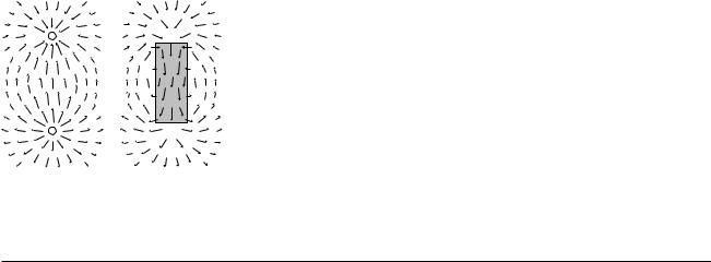
 –
– 
+
(e)(f)
this in terms of more basic principles.
The nonexistence of magnetic monopoles means that unlike an electric field, (e), a magnetic one, (f), can never have sources or sinks. The magnetic field vectors lead in paths that loop back on themselves, without ever converging or diverging at a point.
6.2 Calculating Magnetic Fields and Forces
Magnetostatics
Our study of the electric field built on our previous understanding of electric forces, which was ultimately based on Coulomb’s law for the electric force between two point charges. Since magnetism is ultimately an interaction between currents, i.e. between moving charges, it is reasonable to wish for a magnetic analog of Coulomb’s law, an equation that would tell us the magnetic force between any two moving point charges.
Such a law, unfortunately, does not exist. Coulomb’s law describes the special case of electrostatics: if a set of charges is sitting around and not moving, it tells us the interactions among them. Coulomb’s law fails if the charges are in motion, since it does not incorporate any allowance for the time delay in the outward propagation of a change in the locations of the charges.
A pair of moving point charges will certainly exert magnetic forces on one another, but their magnetic fields are like the v-shaped bow waves left by boats. Each point charge experiences a magnetic field that originated from the other charge when it was at some previous position. There is no way to construct a force law that tells us the force between them based only on their current positions in space.
There is, however, a science of magnetostatics that covers a great many important cases. Magnetostatics describes magnetic forces among currents in the special case where the currents are steady and continuous, leading to magnetic fields throughout space that do not change over time.
If we cannot build a magnetostatics from a force law for point charges, then where do we start? It can be done, but the level of mathematics required (vector calculus) is inappropriate for this course. Luckily there is an alternative that is more within our reach. Physicists of generations past have used the fancy math to derive simple equations for the fields created by various static current distributions, such as a coil of wire, a circular loop, or a straight wire. Virtually all practical situations can be treated either directly using these equations or by doing vector addition, e.g. for a case like the field of two circular loops whose fields add onto one another.
130 |
Chapter 6 Electromagnetism |