Добавил:

Upload Опубликованный материал нарушает ваши авторские права? Сообщите нам.

Вуз:

Уфимский Государственный Авиационный Технический Университет

Предмет:

[НЕСОРТИРОВАННОЕ]

Файл:

lab-inf-4_tasks / 2002_2

.pdf

Скачиваний:

Добавлен:

18.03.2015

Размер:

343.53 Кб

Скачать

☆

1 / 21 2 > Следующая >>>

CMES, vol.3, no.4, pp.465-481, 2002

Temperature Distributions and Thermoelastic Displacements In Moving Bodies

Shuangbiao Liu, Michael J. Rodgers, Qian Wang, Leon M. Keer, and Herbert S. Cheng1

Abstract: Computing the temperature rise and thermoelastic displacement of a material subjected to frictional heating is essential for the realistic modeling of the performance of mechanical components. This paper presents a novel set of frequency-domain expressions for the surface temperature rise and the surface normal thermoelastic displacement of a moving three-dimensional elastic halfspace subjected to arbitrary transient frictional heating, where the velocity of the body and its direction can be an arbitrary function of time. Frequency response functions are derived by using the Carslaw-Jaeger theory, the Seo-Mura result, and the Fourier transform. General formulas are expressed in the form of time integrals, and important expressions for constant body motion velocities are given for the transient-instantaneous, transientcontinuous, and steady-state cases. The thermoelastic responses, in terms of temperature rise and thermoelastic displacement, of the halfspace surface in conﬁgurations similar to pin-on-disk contacts are simulated and discussed.

Nomenclature

			t
d j	Pe j τ dτ ∆ t
		t			2				x
									x
erf x	error function,								exp τ 2 dτ
erf x	error function,								exp τ 2 dτ
					π			0
erfc x complementary error function,
	2			∞
	2			exp τ 2 dτ


i		π x
		π x
	pure imaginary, 1
K	conductivity, J/m ˚ ks or w/m ˚ k
l	characteristic length, m
Pe j	P´eclet number,						j l κ
Pe j	P´eclet number,					V	j l κ
q	heat source, W/m2 or N/ms

1 Center for Surface Engineering and Tribology; Northwestern University; Evanston, IL 60208, USA; 847-467-6961; 847-467-3427 (fax); liusb@northwestern.edu

non-dimensional heat source,

qα t l K

temperature rise, ˚ k

non-dimensional temperature rise, T α t

time, s

l 2

non-dimensional time, κ t

thermoelastic displacement, m

u j

non-dimensional thermoelastic displacement

ﬁeld,

j l 1 ν

velocity in the x j

direction, m/s

frequency domain radius, ω 12 ω 22

effective frequency domain radius,

w2 i ω 1d1 ω 2 d2

coordinate, m

x j

j l

non-dimensional coordinate in j direction, x

α t

linear thermal expansion coefﬁcient, m/m ˚ k

δ i j

Kronecker delta

∆ t

t t

κthermal diffusivity, m2/s

νPoisson’s ratio

ω	1 ω 2	frequency domain counterparts of
ω		x1 x2, respectively
ω	t	counterpart of time in the frequency domain
j		partial derivative with respect to x j coordinate

˜each Fourier Transform

1 Introduction

Frictional heating has been an engineering research topic with a long history. Controlling the effects arising from frictional heating has been a vital part of mechanical engineering design. With the development and constant improvement of computer modeling capabilities, researchers have been able to perform detailed modeling and simulation of frictional heating and contact. Tribological simulations of frictional heating effects include studies on ﬂash temperature [Tian and Kennedy 1994, Qiu and Cheng 1998, and Gao et al. 2000], thermoelastic displacement [Ling and Mow 1965, Barber 1972, Barber 1984, Barber 1987, and Liu et al. 2001], thermoelastic ﬁelds [Ju and Chen 1984, Huang and Ju 1985, Bryant

466

CMES, vol.3, no.4, pp.465-481, 2002

1988, Leroy et al. 1989, Leroy et al. 1990, Ju and Farris 1997, Mow and Cheng 1967, and Ting and Winer 1989], thermoelastic contact [Azarkhin and Barber 1987, Yevtushenko and Kulchytsky-Zhyhailo 1995a, Yevtushenko and Kulchytsky-Zhyhailo 199b, Wang and Liu 1999, Liu and Wang 2000, and Liu and Wang 2001], and thermoelastic instability [Barber 1969, Dow and Burton 1972, Yi et al 1999]. Most of this research is based on the knowledge of heat conduction that is thoroughly and systematically presented by Carslaw and Jaeger’s [Carslaw and Jaeger 1959] (see also [Ling 1973 and Johnson 1996]).

A new approach for calculating the thermoelastic displacement on the surface of an elastic halfspace has been recently developed [Liu et al. 2001], which treats the temperature ﬁeld as an inclusion. Halfspace problems, which are particularly important to Tribology, are solved by using Seo-Mura inclusion theory. Expressions were developed for the thermoelastic displacement in transient-instantaneous, transient-continuous (timeinvariant heat source), and steady-state cases. Frequency response functions (FRFs) for the surface normal thermoelastic displacement were solved [Liu et al. 2001] by substituting the temperature ﬁeld [Carslaw and Jaeger 1959] into the inclusion formula [Seo and Mura 1979], changing the order of integration and applying the Fourier transform and convolution theorem [Press et al. 1992 and Morrison 1997]. These frequency response functions are useful in simulations with arbitrary input because of the recently developed algorithm that uses the fast Fourier transform (FFT) to convert frequency response functions into inﬂuence coefﬁcients and uses discrete convolution and fast Fourier transform (DC-FFT) method to determine the material response [Liu et al. 2000 and Liu and Wang 2002].

In this paper, the new analytical approach [Liu et al. 2001] is extended to obtain a novel set of frequency response functions for the surface temperature rise and the surface thermoelastic displacement in moving threedimensional (3D) elastic halfspace (the coordinate system is ﬁxed to the heat source) subjected to arbitrary transient frictional heating, where the velocity and its direction of the body can be an arbitrary function of time. General formulas are expressed in the form of a time integral, and important expressions are given for the transient-instantaneous, transient-continuous, and steady-state cases. The new formulas allow the fast Fourier transform to be conveniently used to calculate the

thermoelastic responses directly from the applied heat source. As examples, the new formulas are applied to simulate the thermoelastic response of a halfspace with similar conﬁgurations as in pin-on-disk experiments.

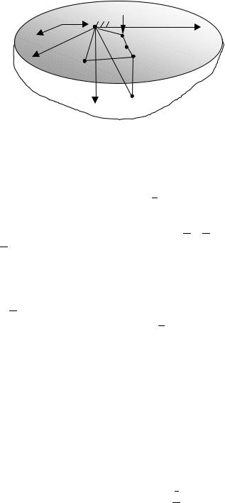
2 Problem Description

		q(x′, x′		,t′)
	Pe1	1	2			1
	Pe1					1
	Pe2		(x′,x′ ,0)
		ρ ′	(x′,x′ ,0)
		ρ ′		1	2
2	(x1 ,x2 ,0)	ρ		(ξ 1 − d1∆ t,ξ 2 − d2 ∆ t,0)
	(x1 ,x2 ,0)			(ξ 1 ,ξ 2 ,0)
				(ξ 1 ,ξ 2 ,0)
				(ξ 1,ξ 2 ,ξ		3 )
		3

Figure 1 : Description of the physcial domain and coordinates

A halfspace (Fig. 1) of a uniform initial temperature distribution is subject to a heat source on the surface. A nondimensional coordinate system x j x j l with characteristic length l is ﬁxed to the heat source, and the halfspace is moving relative to the heat source and the coordinate system along the x j coordinate with speeds (V 1 , V 2, and

V 3 0), which can be functions of time but not space. The material properties of the halfspace are the diffusivity (κ , the linear thermal expansion coefﬁcient (α t , the Poisson’s ratio (ν , and the conductivity (K . The heat source causes a non-dimensional temperature rise T α t T in the halfspace, resulting in a non-dimensional thermoelastic displacement, u j x t u j x t l 1 v

in the x j coordinate direction. The uncoupled governing partial differential equations for transient heat conduction and quasistatic thermoelastic deformation are as follows:

T	∂ T Pe			T	1	Pe	T	2	(1)
ii	∂ t	1			1	2		2
	∂ t
ui j j u j j i 1			2ν			2T i 1 2ν			(2)

where t is the non-dimensional time, t κ t l 2; Pe j is the P´eclet number in the x j direction, Pe j V j l κ ; Roman

Temperature distributions and thermoelastic displacements in moving bodies

467

indices range over 1, 2, 3; the summation convention is

assumed; and j	∂	. The temperature and thermoe-
	∂ x j
lastic boundary conditions for the surface are
Thermal BC:
T 3 q			(3)
Traction free BC:
1 2ν u3 j u j 3 2νδ 3 j uk k 2δ 3 jT			(4)

where the non-dimensional heat source is deﬁned as q x1 x2 t qα t l K for t 0, and q x1 x2 t 0 for t 0. The traction-free boundary condition allows the thermoelastic analysis in this paper to be directly superposed with an isothermal elastic contact analysis [Liu and Wang 2001].

As the heat source may vary with respect to time, the thermoelastic problem may be discussed in three cases accordingly [Barber 1972]: the transient-instantaneous case with a position and time dependent heat source, q x1 x2 t and arbitrary time, the transient-continuous case with position dependent heat source, q x 1 x2 and arbitrary time, and the steady-state case with position dependent heat source, q x1 x2 and t ∞ . Solutions to these heat-source conditions in a moving body offer a general formulation set for the frictional-heating problems.

3 Distribution of Temperature Rise

The solution of Eqs. (1) and (3) for the temperature rise caused by the surface heat source, q x1 x2 t , can be expressed as follows [Carslaw and Jaeger 1959]:

T ξ 1 ξ 2 ξ 3 t

∞

ρ 2 ξ 2

q x

x t

4∆ t

dx dx dt

(5a)

4π 3 2 0 ∞ ∞

∆ t3 2

1 2

where

∆ t

t t ,

the

effective

velocities

are

d j

Pe j τ dτ ∆

and ρ

2 ξ 1

x d1∆

t 2

ξ 2

d2∆

t 2 (Fig.

1).

Equation (5a) can also be

written in a convolution form,

T ξ 1 ξ 2 ξ 3 t t

q ξ 1 ξ 2 t G ξ 1 ξ 2 t t dt

(5b)

with the Green’s function,

G ξ 1 ξ 2 ξ 3 t t

exp

ξ 1 d1∆ t 2 ξ 2 d2∆

t 2 ξ 32

4 ∆ tπ

3 2

4∆

The symbol ‘**’ stands for a two-dimensional (2D) con-

volution. Applying the 2D Fourier transform (FT) with

respect to the ξ 1 and ξ 2 directions, Eqs. (A3) and (A5),

and the convolution theorem (Appendix A), a general

form of the temperature rise in a hybrid domain (fre-

quency, depth and time) is expressed as time dependent

integral,

q˜ ω

1 ω 2 t

exp

ξ 32

∆ tw 2 dt (6)

∆

4∆

Variables ω 1 and ω 2 are the angular frequencies in the

frequency domain; and a double tilde ( ˜ implies a 2D

Fourier transform. The frequency domain radius is w

22 , and the effective frequency domain radius is

w2 i ω

1d1 ω

2 d2

. If the P´eclet numbers (or

velocities,

1 and

2 vary with time, numerical integra-

tion must be used for the effective velocities d j and for

Eq. (6) to evaluate the time integrals. In the following,

important formulas with time-invariant P´eclet numbers,

i.e., d j Pe j = constant, are discussed.

Transient-Instantaneous Case.

Since

the

heat

source

q˜ ω

1 ω 2 t and

the

function

g˜ ω

1 ω

2 ξ 3 t

exp ξ43t

tw 2

are zero when t 0, Eq. (6) is a

convolution related to the Fourier transform with respect

to t, and can be expressed as (see Eq. (A8))

ω t

exp

ξ 3

iω

(7)

q˜ ω 1 ω 2 ω t

w 2 iω t

where ω t is the frequency domain counterpart of time,

and a triple tilde ˜ implies a 3D Fourier transform. The

right-hand side of Eq. (7) is the corresponding frequency

response function (FRF) for transient-instantaneous tem-

perature rise, which gives the temperature rise caused by

an instantaneous point heat source.

Transient-Continuous Case If the heat source is not a

function of time, Eq. (6) can be written as

q˜ ω 1 ω

2 t

2 2

dτ

(8)

2 exp

4τ 2

468 Copyright c 2002 Tech Science Press

with τ

. Therefore,

∆ t

T ω

ω 2

ξ 3

(9)

q˜ ω

1 ω

w 0

3 w

ξ 3

ξ 3 w

ξ 3

erfc

2 t

w t e

erfc

2 t

w t Æ 2w

w 0

2exp ξ 32

π ξ 3 erfc

ξ 3

2 t

The right-hand side of Eq. (9) is the frequency response function for transient-continuous temperature rise, which gives the temperature rise caused by a continuous point heat source. If the velocities are not zero, Eq. (9) includes a complementary error function erfc x with complex arguments and can be evaluated by using a special function, ϖ z [Abramowitz and Stegun 1964, Appendix B]. The solution in Ting and Winer’s paper [1989] is a stationary case of Eq. (9).

Steady-State Case The frequency response function for steady-state temperature rise is found from Eq. (7) by

letting ω

0, or from Eq. (9) by letting t ∞ ,

ω 1

ξ 3

ξ 3 w

(10)

q˜ ω 1 ω 2

Again, note that Eqs. (7), (9 and (10) are only valid for constant P´eclet numbers (velocities).

4 Normal Surface Thermoelastic Displacement

The solution of Eqs. (2) and (4) for the quasi-static thermoelastic displacement is found from the Green’s function for a point force in the interior of a halfspace [Mindlin 1953], using the approach of Seo and Mura [1979]. The normal surface thermoelastic displacement is given by [Liu et al. 2001]

x x 0 t 1

(11)

∞

ξ 3

∞ T ξ 1 ξ 2 ξ 3 t

dξ 1 dξ 2dξ 3

∞

ρ 2 ξ

3 2

where ρ 2

x1 ξ

x2 ξ 2 . Similar to Equations

(5), the convolution theorem and Eq. (A6) are used to take the 2D Fourier transform of Eq. (11), giving

CMES, vol.3, no.4, pp.465-481, 2002

u˜3

∞

ξ 3w

dξ 3

(12)

ω 1 ω

0 t

ω 1 ω

ξ 3 t exp

Substituting Eq. (6) into Eq. (12) gives

u˜3 ω 1 ω 2

0 t

∞ t

2 t 1

q˜ ω

1 ω

exp

ξ 3

∆ tw 2 ξ 3 w dt dξ 3

(13)

4∆ t

∆

Interchanging the order of integration allows the depth integral to be performed analytically, resulting in the following compact form

u˜3 ω 1 ω 2 0 t 2

(14)

q˜ ω 1 ω 2 t exp i∆ t ω 1d1 ω 2d2 erfc w ∆ t dt

which is the general form of the normal surface thermoelastic displacement expressed in a hybrid domain (frequency and time). If the P´eclet numbers vary with time, numerical integration must be used to evaluate the time integrals for the effective velocities d j and for Eq. (14). However, important formulas with constant P´eclet numbers are further discussed below.

Transient-Instantaneous Case. For the transientinstantaneous case with constant P´eclet numbers, Eq. (14) is treated as a convolution related to the Fourier transform with respect to t. Applying the convolution theorem, the frequency-shift property of the Fourier transform, and Eq. (A7) gives

u˜3 ω 1 ω 2 0 ω t		2	(15)

q˜ ω 1 ω 2 ω t	iω t w 2 iω t w 2 w

Therefore, the corresponding frequency response function, which gives the displacement caused by an instantaneous heat source, is given by the right-hand-side of Eq. (15) with a singularity when both w = 0 and ω t = 0 (note that w = 0 when w = 0).

Transient-Continuous Case. If the P´eclet numbers are constant and the heat source is not a function of time, Eq. (14) is written as

Temperature distributions and thermoelastic displacements in moving bodies

469

u˜3 ω 1 ω 2 0 t 2q˜ ω 1 ω 2
0t	exp i ω 1d1 ω 2 d2 τ erfc w τ dτ	(16)

Eqs. (14 - 18) reduce to the results given by [Liu et al. 2001]. It should be pointed out that the entire thermoelastic displacements at any interior location of the halfspace could be obtained following the same derivation process.

Numerical Methods

Equation (16) is integrated, and the frequency response

For problems with an irregular heat source, the discrete

function for the transient-continuous case is given by the

convolution and fast Fourier transform algorithm [Liu

right-hand-side of

and Wang 2002] may be used to obtain efﬁcient and accu-

rate results. The inﬂuence coefﬁcients [Johnson 1996] of

u˜3 ω

1 ω

2 0 t

the responses (temperature rise and normal surface ther-

moelastic displacement) are essential in this algorithm.

q˜ ω 1 ω 2

If the heat source has a known Fourier transform, the re-

2i 1 exp ω 1d1 ω

sponses can be obtained from Eqs. (6), (7), (9) or (10)

2 d2 it erfc w t

and Eqs. (14), (15), (17) or (18) by inverse Fourier trans-

w erf w

w ω

1d1 ω 2d2

(17)

form, which could be numerically calculated in several

ways.

In this paper,

the conversion process [Liu and

Wang 2002] with inverse fast Fourier transform (FFT)

The frequency response function gives the displacement

algorithm is used, which is an essential part to obtain

the inﬂuence coefﬁcients in the discrete convolution and

caused by a continuous heat source. When the veloci-

fast Fourier transform algorithm. Given the intervals (∆ 1

ties are zero, Eq. (17) does not apply; instead, Eq.

(16)

should be integrated for that case (the result is given in

and ∆ 2for x1 and x2 directions) in the space domain, fre-

[Liu et al. 2001]). At w = 0, the frequency response

quency response functions are truncated between nega-

tive and positive Nyquist frequencies ( π /∆ 1 and π /∆ 2

function is ‘–2t’, and therefore it has no singularity. The

frequency response function includes an error function

for ω 1 and ω 2 directions). If the space and frequency do-

erf x with complex arguments, which again can be eval-

mains have the same number of discrete points (N1 and

uated by using the special function ϖ z [Abramowitz and

N2 for x1 and x2 directions, and for ω 1 and ω 2 directions),

Stegun 1964, Appendix B].

the aliasing error in the results obtained by the conver-

sion process may become signiﬁcant. In order to reduce

Steady-State case.

When steady-state conditions pre-

the aliasing error, the number of discrete points in the fre-

vail, Eq. (16) is integrated analytically, and the frequency

quency domain should be large enough. In this paper, the

response function for the steady-state case is given by the

number of discrete points in the frequency domain are

right-hand-side of

8N1 and 8N2 in the ω 1 and ω 2 directions, respectively,

and this choice has the effect of reﬁning the interval in

u˜3 ω

1 ω

2 0

(18)

the frequency domain for sufﬁciently accurate results.

q˜ ω

1 ω

w w

Since the complementary error function and error func-

which is a special case of the transient frequency re-

tion require a signiﬁcant amount of computation, the

following approximations are used to save computation

sponse function from Eq.

(15) with ω t 0, and has a

time, erfc x 3 0

erf x 3 1. Standard Gaus-

singularity at w = 0. One of the striking properties of fre-

sian quadrature is used to carry out the numerical inte-

quency response functions is that the frequency response

gration in Eqs. (6) and (14), when numerical integration

functions in a plane-strain problem are simply those in a

is necessary.

three-dimensional problem with ω 2 = 0 [Liu and Wang

2002]. Equation (18) with ω 2 0 agrees with the 2D re-

Numerical Simulations

sult obtained by Bryant [1988] or Ju and Farris [1997].

Note that Eqs. (15 – 18) again are valid only for constant

The formulations developed in Sections 2-4 enable nu-

P´eclet numbers. If the speeds are zero, the expressions in

merical

simulation of the thermoelastic response of a

470

CMES, vol.3, no.4, pp.465-481, 2002

Pe1= Constant

1
2
(a)
Pe1(t)
Pe2(t)
1
2
(c1)

Pe1(t)

(b)

Pe1(t)

Pe2(t)

(c2)

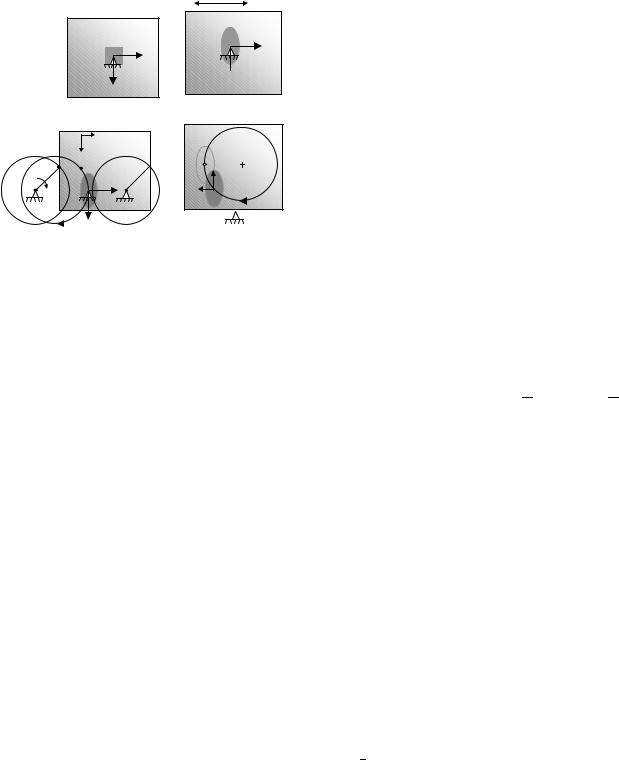
Figure 2 : Three translation motions of a halfspace (a) A rectangular heat source on a a pure translating halfspace. (b) An elliptical heat source on a reciprocating halfspace. (c1) An ellipitical heat source on a circularly translating halfspace. (c2) A circularly translating elliptical heat source on a ﬁxed halfspace, which is equivalent to (c1).

halfspace by computing the transient three-dimensional temperature rise ﬁelds and normal surface thermoelastic displacement. Three example cases are numerically solved to illustrate the use of the formulations, where three different motions of the halfspace are speciﬁed to show the novelty of the formulations: pure translation (Fig. 2(a , reciprocating translation (Fig. 2(b , and circular translation (Fig. 2(c1)). It should be pointed out that the three examples do not directly correspond to the three cases of heat source, and frequency response functions of Eqs. (7) and (15) for transient-instantaneous cases with a constant P´eclet number are not exempliﬁed in this paper. However, in pure translation, both transient-continuous and steady-state case are studied; in reciprocating translation, the transient-instantaneous case, which uses the general equations (6) and (14), is studied; in circular translation, the transient-continuous case is studied. In the latter two examples, the steady state results may not exist. In each simulation, a known heat source is given with regard to the coordinate system, which is ﬁxed to the heat source. The values of velocities, characteristic lengths and material properties are chosen from a typical counterformal contact in tribological applications [Liu and Wang 2001]. Other parame-

ters are chosen for the convenience. The temperature rise and the normal thermoelastic displacement are obtained on the surface discretzied with 128 128 rectangular elements, which is sufﬁcient to give smooth results in all the cases studied. Note that the x2 coordinates in Figs. 2 are downward to be consistent with Fig. 1. However, in all contour plots, x2 are upward for the observation convenience. Also in all contours plots the interval between contours is ﬁxed and the limits of axes are chosen to show results in a better focus. Although results are presented within only a single cycle for the latter two examples, it should be pointed out that the responses at any cycle or time could be calculated from the initial uniform state (nonuniform initial temperature condition is not explored in the current study) provided that the Gaussian integration is sufﬁciently accurate.

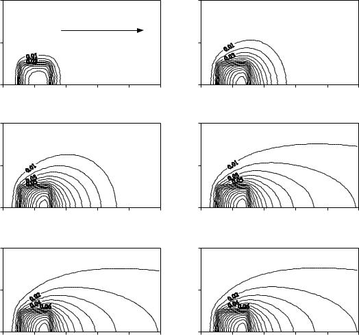
6.1 Pure Translation

Figure 2(a describes the conﬁguration with a constant heat source q 1, over a region of x1 1 4 1 4 , x2 1 4 1 4 . The constant P´eclet numbers are Pe1 10 Pe2 0, which correspond to V 1=1 m/s and V 2 = 0 m/s at l = 1 mm and κ =10 4 m2/s. Results are computed in the region of x1 2 2 , x2 2 2 . The Nyquist critical angular frequencies in both directions are 32π . The temperature rise and the displacement are calculated with Eqs. (9 – 10) and with Eqs. (17 – 18), respectively. The results are plotted in Figs. 3 – 4 to show the evolution to steady state. Not surprisingly, the tails of both temperature and displacement distributions resemble wakes and spread outward perpendicular to the direction of motion and along the motion direction of the body. Because the temperature rise is directly related to the heat source, sharp temperature gradients appear around the border of the heat-application area, corresponding to the discontinuity of the heat source, as shown in Fig. 3. However, the temperature rise in the entire body causes the surface to deform, and the contours for the displacement distribution look smoother than those of the temperature rise, as shown in Fig. 4. Figures 5 and 6 further compare the responses along the line of x2 = 0 at different times (t=0.01t . The responses start from a nearly symmetric peak localized with respect to the region of the heat source application. Increasing the time of heating causes their peaks to rise due to the heat accumulation in the solid even though new parts of the surface continuously pass by the heat source. As a result of the halfspace

Temperature distributions and thermoelastic displacements in moving bodies

471

1.0
	x2		t = 0.01
			t = 0.01
0.5			Direction of body’s motion
0.5
						x1
0.0
-0.5		0.0	0.5	1.0	1.5	2.0
			(a)
1.0	x2		t = 0.1
			t = 0.1

0.5
						x1
0.0
-0.5		0.0	0.5	1.0	1.5	2.0
			(c)
1.0	x2		t = 1
			t = 1
0.5
						x1
0.0
-0.5		0.0	0.5	1.0	1.5	2.0
			(e)

1.0
	x2		t = 0.05
			t = 0.05
0.5
						x1
0.0
-0.5		0.0	0.5	1.0	1.5	2.0
			(b)
1.0	x2		t = 0.5
			t = 0.5
0.5
						x1
0.0
-0.5		0.0	0.5	1.0	1.5	2.0
			(d)
1.0	x2		Steady-state
			Steady-state
0.5
						x1
0.0
-0.5		0.0	0.5	1.0	1.5	2.0
			(f)

Figure 3 : Contours of the distributions of the surface temperature rise, T x 1 x2 0 t , of the purely translating halfspace (Fig. 2(a)). Here, (a) through (f) show the evolution as time increases, and (f) shows the stead-state case.

472

CMES, vol.3, no.4, pp.465-481, 2002

1.5			1.5
1.5	x2	t = 0.01	1.5	x2	t = 0.05
	x2			x2

1.0			1.0

Direction of body’s motion

0.5								0.5
0.0							x1	0.0							x1
0.0								0.0
-1.0		-0.5	0.0	0.5	1.0	1.5	2.0	-1.0		-0.5	0.0	0.5	1.0	1.5	2.0
				(a)								(b)
1.5	x2			t = 0.1				1.5	x2			t = 0.5
				t = 0.1								t = 0.5
1.0								1.0
0.5								0.5
							x1								x1
0.0								0.0
-1.0		-0.5	0.0	0.5	1.0	1.5	2.0	-1.0		-0.5	0.0	0.5	1.0	1.5	2.0
				(c)								(d)
1.5	x2			t = 1				1.5		x2	Steady-state
				t = 1							Steady-state
1.0								1.0
0.5								0.5
							x1								x1
0.0								0.0
-1.0		-0.5	0.0	0.5	1.0	1.5	2.0	-1.0		-0.5	0.0	0.5	1.0	1.5	2.0
				(e)								(f)

Figure 4 : Contours of the thermoelastic displacements, - u 3 x1 x2 0 t , of the pure translating halfspace (Fig. 2(a)). Pe1 = 10, and Pe2 = 0. Here, (a) through (f) show the evolution as time increases, and (f) shows the steadystate case.

Temperature distributions and thermoelastic displacements in moving bodies

473

translating to the positive direction of x 1, the responses in the positive side of x1 becomes larger than those in the negative side of x1. Therefore, the maximum values are found at positions in the positive side of the origin. The 2D steady state result corresponding to a heat source that has the same width of application as that of the 3D heat source used in this case is also calculated and shown in Fig. 5. The 2D steady-state temperature rise is higher than the 3D steady-state result because the heat source for the 2D solution is a line source (with the same width but with inﬁnite length), and therefore the quantity of heat input is much higher for the 2D case.

	1E-1
	1E-2	Time t
t)		∞
0,	1E-3	1
, 0,		1
, 0,		0.5
1		0.1
x		0.1
(	1E-4	0.05
3	1E-4	0.05
-u
	1E-5	0.01
	1E-5
		Direction of body’s motion
	1E-6
	-2	-1	0	1	2
			x1

	0.25							Figure 6 : Thermoelastic displacements of the surface of
								Figure 6 : Thermoelastic displacements of the surface of
				Direction of body’s motion				the halfspace under a pure translation motion at different
	0.20			Direction of body’s motion				times.
	0.20							times.
t)	0.15								b
0,	0.15								b
0,								10
0,								10
0,								a	c
1								Pe1
,
(x	0.10
T						2D, t = ∞
						2D, t = ∞			d	h
								0
	0.05
		t =	0.01	0.05	0.1	0.5, 1, ∞			e	g
									e

	0.00							-10		f
	-0.5	0.0		0.5	1.0	1.5	2.0	-10
	-0.5	0.0		0.5	1.0	1.5	2.0				t
								0.0	0.3	0.6	t
				x1

Figure 5 : Temperature rises on the surface of the halfspace under a pure translation motion at different times.

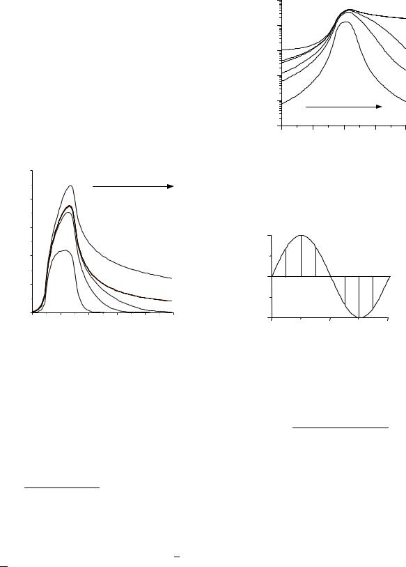
Figure 7 : Variation of the x-direction P´eclet number for case B for the reciprocating halfspace.

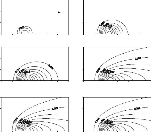
6.2 Reciprocating Translation

Fig. 2(b describes a reciprocating halfspace subjected to a stationary heat source that corresponds to the Hertzian


pressure distribution p	c 1 x	1	c 2 x c			2	2
		1	1		2	2
with c1 0 25 c2 0 5,	and c K α			tκ ,	whose
Fourier transform pairs is 2π	c c1c2 sinΘ		Θ	cos Θ	Θ	3

with Θ ω 1c1 2 ω 2c2 2. The heat source has an elliptical base with a center at the origin, and two different elliptical radii are chosen to identify directions. The halfspace is translating with a sinusoidal P´eclet number, Pe1 t 10 sin 2π t 0 6 (Fig. 7).

The dimensional heat source is deﬁned as, q µ f p r V 1 t , a function of both position and time, where the constant frictional coefﬁcient, µ f , is 0.1. Therefore,

q sin 2π t 0 6 1 x1 c1 2 x2 c2 2. Both surface temperature rise and normal surface thermoelastic displacement of the halfspace are calculated in the region of x1 4 4 and x2 3 3 using Eqs. (6) and (14), and the results are plotted in Figs. 8 and 9, respectively. In these two ﬁgures, (a through (h correspond to the positions a through h on the sinusoidal P´eclet-number curve shown in Fig. 7. The motion direction directly inﬂuences the contour spreading direction and the location of the maximum value, which is not at the origin again. Figures 8(e and 9(e , which show the results after the motion direction is reversed, clearly indicating the residual ﬁelds of the responses from the previous motion.

474

CMES, vol.3, no.4, pp.465-481, 2002

1.0	x2			t = t0/8		1.0	x2				t = 2 t0/8
0.5			0.04			0.5					0.04
					x1						0.04	x1
											0.08
											0.08
0.0						0.0					0.12
0.0						0.0
-2.0		-1.0	0.0	1.0	2.0	-2.0		-1.0	0.0		1.0	2.0
			(a)						(b)
1.0	x2			t = 3 t0/8		1.0	x2				t = 4 t0/8
				t = 3 t0/8							t = 4 t0/8
0.5						0.5					0.04
				0.04	x1						0.04	x1
			0.12	0.04	x1					0.12	0.08	x1
0.0			0.12	0.08		0.0				0.12
0.0						0.0
-2.0		-1.0	0.0	1.0	2.0	-2.0		-1.0	0.0		1.0	2.0
			(c)						(d)
1.0	x2			t = 5 t0/8		1.0	x2				t = 6 t0/8
				t = 5 t0/8							t = 6 t0/8
0.5						0.5		0.04
			0.04		x1			0.08				x1
					x1							x1

0.0						0.0		0.12
0.0						0.0
-2.0		-1.0	0.0	1.0	2.0	-2.0		-1.0	0.0		1.0	2.0
			(e)						(f)
1.0	x2			t = 7 t0/8		1.0	x2				t = t0
				t = 7 t0/8							t = t0
0.5		0.04				0.5		0.04
		0.04			x1			0.04				x1
		0.08 0.12			x1			0.08				x1
0.0						0.0		0.12
0.0						0.0
-2.0		-1.0	0.0	1.0	2.0	-2.0		-1.0	0.0		1.0	2.0
			(g)						(h)

Figure 8 : Contours of the distributions of the surface temperature rise, T x 1 x2 0 t ,on the surface of the reciprocating halfspace (Fig. 2(b)). Here, (a) through (h) are corresponding to positions ’a’ through ’h’ on the sinusoidal P´eclet-number curve shown in Fig. 7.

1 / 21 2 > Следующая >>>

Соседние файлы в папке lab-inf-4_tasks

#
18.03.2015172.41 Кб172.pdf
#
18.03.20151.01 Mб192000_34.pdf
#
18.03.2015645.78 Кб182000_521.pdf
#
18.03.2015252.92 Кб172001.pdf
#
18.03.2015692.17 Кб172002.pdf
#
18.03.2015343.53 Кб172002_2.pdf
#
18.03.2015219.18 Кб172777.pdf
#
18.03.2015694.06 Кб234N.pdf
#
18.03.2015367.37 Кб176164.pdf
#
18.03.2015422.77 Кб177918.pdf