lab-inf-4_tasks / 2

ABSTRACT

This paper demonstrates the importance of taking statistical process variations into account when designing semiconductor processes, and provides a methodology for doing so. An on-axis, high-energy ion-implant process is used as a vehicle to demonstrate the methodology. UTMARLOWE is the well-calibrated (and hence predictive) simulation tool of choice. It is shown that crystal-cut errors and implanter-tilt errors can result in a considerably off-axis implant for this nominally on-axis implant: instead of the intended tilt = 0°, the implant actually occurs at an average tilt of ~0.65°, with a significant probability of having tilt > 1°. Knowledge of the error-statistics is used to design a robust process (i.e. a process relatively immune to statistical process variations), thereby providing better control over device performance. This methodology can also account for deterministic errors arising from beam divergence and processdisk geometry in multi-wafer machines.

Keywords: Statistical-process-error, ion-implantation, tilt, angle, process-design

1 INTRODUCTION

Predictive simulation of processes such as ionimplantation is important in technology development [1-2]. UT-MARLOWE, a state-of-the-art Monte-Carlo simulator [3], is found to be very accurate in Motorola for simulating implant profiles at various energies, and is thus considered to be predictive, especially for high-energy profiles in the sub1MeV range.

An on-axis (tilt=0°), 750keV, phosphorus implant through a ~60Å screen oxide is used as a case-study. As shown in Fig. 1, UT-MARLOWE predicts a second (deeper) peak which is not seen in the SIMS data; this spurious doping peak can strongly affect simulated electrical characteristics of certain devices. Such errors in predicted profiles must therefore be avoided. We find that the discrepancy actually arises from random fabrication process errors neglected till now. These errors are described in the next section.

Crystal-cut error is measured using x-ray diffractometry, and is quantified as two tilt-angles about orthogonal axes A and B [4], as illustrated in Fig. 2. This error can thus be represented by random variables (RVs) CUTA and CUTB. Statistics for the two RVs are summarized in Table 1 [4]. Evidently, the statistical distribution is very tight, i.e. s-values are very small.

Table 1. Crystal-cut error statistics from two lots of seventy-five (100)-oriented wafers [4]. XRD is used to determine the rotation of the [100] vector about axes A and B of Fig. 2.

Crystal-Cut (Slice Alignment) error about axes A and B

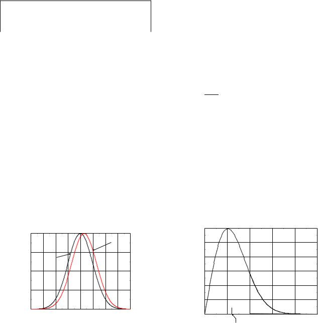
In addition, misalignments in the implanter can lead to random errors in the tilt angle. These misalignments are measured about the same axes A and B. For low tilt angles, the expected best-case accuracy is ± 0.5° about each axis. This implies two RVs, IMPLANTERA and IMPLANTERB, each with a mean=0° and s=0.5°. Given only the mean value and standard deviation for an RV, it is necessary to assume a Gaussian probability density for it [5]. Consequently, Gaussian density functions are assumed for the four RVs: CUTA,B and IMPLANTERA,B, with the mean and s values mentioned above. For axis A, the total tilt angle (QA) is therefore a RV equal to the sum of CUTA and IMPLANTERA, and similarly for QB. It is easily shown that the sum of two Gaussian RVs is also a Gaussian RV [6]. Therefore QA and QB are also Gaussian RVs [6], with probability densities described in Eqn. 1 and plotted in Fig. 3.

meanA = mean[ A] = mean[CUTA] + mean[IMP LANT ERA], &

Equation 1. Mean and std.-deviation for the total tilt about axis A, which is a Gaussian RV given by

QA = CUTA + IMPLANTERA. Similarly for QB.

Figure 3. Gaussian probability density functions for the RVs QA and QB as in Equation 1. For this particular case, s(QA) = s(QB) » 0.5°.

It must be noted that tilt and rotation angles commonly used during wafer-processing or implant-simulation, are actually referred to the polar co-ordinate system. It is easily shown using geometrical analysis that for small tilt angles, tilt (Q) and rotation (F) are given by (Q)2 = (QA)2 + (QB)2, and F = QB/QA. From these two relationships, the probability density functions for Q and F (both of which are RVs) may easily be derived [6]. The probability density function for Q is described in Eqn. 2. Here m2 = (meanA)2 + (meanB)2, s = sA = sB and Io(x) is the modified Bessel function of zeroth order.

Equation 2. Rayleigh-like probability density for random variable Q, using (Q)2 = (QA)2 + (QB)2.

Also see Fig. 4(a).

Equation 3. Cauchy-like probability density, for F = QB/QA [6], plotted in Fig. 4(b).

Note that since m ¹ 0, pΘ(q) is not a true Rayleigh function; however it does have Rayleigh-like characteristics. Eqn. 3 describes the Cauchy-like probability density function, pΦ(f), for rotation angle F. Note that for this case meanA and meanB are non-zero, and therefore analytical solutions for pΘ and pΦ are not obtainable. As a result the symbolic equation solver, MathematicaTM was used to calculate the functions. These have been plotted in Fig. 4(a) and Fig. 4(b). Incidentally, if meanA = meanB = 0, pΦ(f) is a true Cauchy function, given by pΦ(f) = 1/(p + p f2).

Please see Table 2 for some important properties.

It is evident (see Fig. 4(a)) that for the nominally 0° tilt implant, the average tilt is actually 0.638°. The area under the probability density function for 1°<θ<∞ is the probability that θ>1°; it is clear that there is a significant probability (14.5%) for this to occur. If realistic values of implanter inaccuracies are assumed instead of the best-case values, this probability rises even higher. This is summarized in Fig. 5.

Figure 4(b). Cauchy-like pF(φ), from Eqn. 3. The area under the visible part of the curve is

PF(-10° ≤ φ ≤ +10°) = 93.4%.

Figure 5. Mean value for Θ, and P(θ > 1°) for lot #1. For σ=1°, P(θ > 1°)=61%. Note that for a Rayleigh-distributed RV, the mean value depends linearly on the σ of the underlying Gaussian RVs.

This is why in Fig. 6 there is a good match between the SIMS measurement and simulation, to a depth of ~2.0μm using a tilt=1°. Note that there is still a discrepancy in the tail region between measurement and simulation. This is partly due to a lack of significant statistics (in the Monte Carlo simulation) at that depth. In addition, there are two other possibilities: the neglect of damage due to electronic stopping and secondly, electron gas polarization, which causes implanted ions to experience a non-isotropic and nonuniform force presently ignored in the simulator [3].

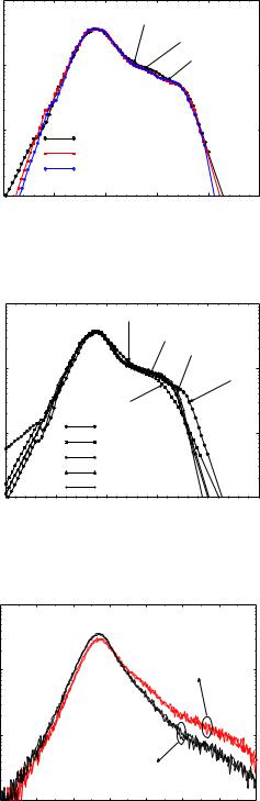
beam divergence and the wafer size, it is possible to introduce a suitable correction to mean-values of pΘ and pΦ. These corrections are in general dependent on the nominal tilt and rotation angles.

Figure 7(a). UT-MARLOWE simulations for various values of φ, with θ=1°. The lack of variability indicates nominal φ=0° for robustness.

4 CONCLUSIONS

It has been shown using probability theory that the discrepancy between SIMS measurement and simulated profiles for the example 750keV phosphorus implant is due to a ~1° error in the implant angle. This is due to random errors in the crystal cut and implanter alignment, previously unaccounted for. Even with the availability of an accurate implantation simulator, implant errors have to be rigorously accounted for in order to be predictive. Differences in implanted profiles can translate to differences in electrical performance. For instance, if this phosphorus implant formed the n-well region for a PMOS transistor, the wellsubstrate junction profile and hence the electrical properties of this junction (such as leakage current and breakdown voltage) become strongly dependent on the actual tilt-angle in the implant process. Therefore, for a repeatable process, it is necessary to carefully design the process using the methodology outlined in this work. For the example chosen, the nominally "on-axis" implant has to be centered around θ=4°,

φ=0°.

The industry increasingly relies on TCAD methods for reducing technology development costs. This work illustrates the power of introducing statistical methods into traditional TCAD activity. Such a merging of disciplines can benefit not only technology development but also metrology.

ACKNOWLEDGMENTS

We thank Craig Jasper, Colin McAndrew and Charly Wimmer of Motorola, Borna Obradovic of the University of Texas, Tom Mercer and Ken Myers of MEMC Corporation and Gerhard Hobler of AT&T for helpful discussions. Steve Merchant provided valuable help with MathematicaTM.

REFERENCES

[1]S. Morris, et al, IEEE-IEDM Technical Digest, p. 721-724, 1996.

[2]G. Hobler, et al, IEEE-IEDM Technical Digest, p. 489-492, 1997.

[3]UT-MARLOWE manual, University of Texas at Austin and Los Alamos National Labs.

[4]Data from MEMC Electronic Materials, Inc.

[5]J.N. Kapur & H.K. Kesavan, "Entropy Optimization Principles with Applications," Academic Press, p.62, 1992.

Figure 8. SIMS data for a 2MeV, on-axis phosphorus implant. Tilt-angle at the edge is quantifyably and deterministically larger than at the center.

[6] Athanasios Papoulis, "Probability, Random Variables, and Stochastic Processes," McGraw-Hill, 1984.