

lab-inf-4_tasks / 2002
.pdfVol. 45 No. 4 |
SCIENCE IN CHINA (Series E) |
August 2002
Simulation of temperature distribution of point contacts in mixed lubrication
LIU Yuchuan ( |
), HU Yuanzhong ( |
), WANG Wenzhong ( |
) |
& WANG Hui ( |
) |
|
|
State Key Laboratory of Tribology, Tsinghua University, Beijing 100084, China Correspondence should be addressed to Liu Yuchuan (email: liuyc@pim.tsinghua.edu.cn)
Received December 19, 2001
Abstract The numerical simulation of temperature distribution of point contacts in mixed lubrication is presented. The calculating includes two steps. First, temperature rises on two surfaces are obtained by a temperature integration method of transient point heat source. Second, the partition coefficients of heat flux are determined by matching the temperature of two surfaces. Similar to the calculation of elastic deformation, double linear interpolation function is used to get a better accuracy, and moving grid method is used to increase the efficiency of the computation. Due to the symmetry of influence coefficient matrix in the direction perpendicular to the velocity, storage and computational work are further reduced by 50%. Numerical samples validate the algorithm and program. The calculating results of the cases of smooth surface and isotropic sinusoidal surface are presented.
Keywords: temperature, point contacts, mixed lubrication.
The friction-originating temperature rise on solid bodies is the sum of flash temperature and bulk temperature[1]. Bulk temperature is easy to measure, but flash temperature is difficult to measure as it is transient and only lasts a very short time. So only numerical method can be used to obtain flash temperature distribution. Today the numerical simulation of tribology has been gereralized from full film elastohydrodynamic lubrication on smooth surfaces to mixed lubrication on real rough surfaces. To deeply analyze the mechanisms of sliding failure under real conditions the simulation of temperature distribution in mixed lubrication becomes a hot issue now.
The foundation of any temperature field calculation is heat conduction equation for solid and
Nomenclature a, Hertzian contact radius; c, specific heat of solid; C1,C2, influence coefficients of body 1 and body 2; f,
heat partition coefficient; h , |
h |
, oil film thickness and its dimensionless parameter, |
|
h |
h / a ; Ks, Kf , thermal conductivities of |
||||||||||||||||||||||||||||||||||||||||||||||||||||||||||
solid and fluid; p, |
p |
, pressure and its dimensionless parameter, |
p |
p / ph ; ph= maximum Hertzian pressure, |
q , |
q |
, heat flux |
||||||||||||||||||||||||||||||||||||||||||||||||||||||||
density and its dimensionless parameter, q pV , |
|
|
|
|
; S 3/ 2K |
|
/ K |
|
; |
t, |
|
|
|
|
|
|
|
|
|
|
|||||||||||||||||||||||||||||||||||||||||||
|
|
|
|
|
, time and its dimensionless parameter, |
||||||||||||||||||||||||||||||||||||||||||||||||||||||||||
q |
pV |
s |
f |
t |
|||||||||||||||||||||||||||||||||||||||||||||||||||||||||||
|
|
|
|
|
|
|
|
|
|
|
|
|
|
|
|
|
|
|
|
|
|
|
|
|
|
|
|
|
|
s |
|
|
|
s |
|
|
|
|
|
|
|
|
|
|
|
|
|
|
|
|
|
|
|
|
|
|
|
|
|
||||
|
|
|
|
t 4 / a2 ; |
T |
,T |
|
|
|
|
|
|
|
|
|
|
|
|
|
|
|
|
|
|
|
|
|
|
|
|
|
T 3/ 2 c /(2p ) ; |
|||||||||||||||||||||||||||||||
|
t |
|
, T |
|
,T |
, bulk temperatures of body 1 and body 2 and the dimensionless forms, T |
|||||||||||||||||||||||||||||||||||||||||||||||||||||||||
|
|
|
|
|
|
|
|
|
|
|
|
|
|
|
|
1b |
|
|
2b |
|
1b |
|
2b |
|
|
|
|
|
|
|
|
|
|
|
|
|
|
|
|
|
|
|
|
|
|
|
|
|
|
|
|
|
|
|
|
|
|
|
h |
||||
|
|
|
|
|
|
|
|
|
, dimensionless temperatures rises of body 1 and body 2; u |
|
|
|
|
|
|
|
|
|
|
|
|
|
|
|
|
||||||||||||||||||||||||||||||||||||||
T |
, T |
t |
|
t ; |
|
V ,V ,V ,V = velocities of body 1 and body 2 |
|||||||||||||||||||||||||||||||||||||||||||||||||||||||||
1 |
2 |
|
|
|
|
|
|
|
|
|
|
|
|
|
|
|
|
|
|
|
|
|
|
|
|
|
|
|
|
|
|
|
|
|
1 |
2 |
1 |
2 |
|
|
|
|
|
|
|
|
|
||||||||||||||||
and |
the |
dimensionless |
|
|
|
|
|
velocity and |
|
its |
|
dimensionless parameter, |
Vs |V1 V2 | , |
||||||||||||||||||||||||||||||||||||||||||||||||||
forms, V |
Va /(4 ) ; Vs ,Vs , sliding |
|
|
||||||||||||||||||||||||||||||||||||||||||||||||||||||||||||
|
|
|
|
|
|
|
|
|
|
|
|
|
|
|
|
|
|
|
|
|
|
|
|||||||||||||||||||||||||||||||||||||||||
Vs |
|V1 |
V2 | ; |
x, y, |
x |
, |
y |
, Cartesian coordinates and |
nondimensional, |
x |
x / a , |
y |
y / a ; |
x |
, |
y |
, mesh |
spacing in the |
||||||||||||||||||||||||||||||||||||||||||||||
direction of |
x |
and |
y |
axis; Ks / c , thermal diffusivity of solid; , friction coefficient; , density of solid; , solution |
|||||||||||||||||||||||||||||||||||||||||||||||||||||||||||
domain; Pe=Va /(2 ) , Peclet number. |
|
|
|
|
|
|
|
|
|
|
|
|
|
|
|
|
|
|
|
|
|
|
|
|
|
|
|
|
|
|
|
|
|||||||||||||||||||||||||||||||
366 |
SCIENCE IN CHINA (Series E) |
Vol. 45 |
energy equation for fluid. For hydrodynamic and elastohydrodynamic lubrication, the most accurate method is using finite difference method and simultaneously solving the heat conduction equation of solid surfaces and energy equation of fluid for given boundary conditions[2 4]. In the case where surface temperature is a major concern, a surface temperature equation[5] has been widely employed[6 8]. But the equation is based on the assumption that the heat source moves very fast. If one surface is stationary with respect to heat source, the use of surface temperature equation will bring about big computational errors.
For dry contact and boundary lubrication without hydrodynamic film, the moving point heat source integration method described in ref. [5] is often used. By integrating the analytic solution with respect to appropriate time and spatial variables for a given geometry and heat intensity, the transient and steady state solutions can be obtained. Using this method, refs. [9 11] studied the steady state flash temperature of various heat sources at different Peclet numbers. As a matter of fact, surface temperature equation is a deduction of this method under the condition of high Peclet number.
A major feature of mixed lubrication is the coexistence of both hydrodynamic lubrication area and dry contact area. The calculation of temperature field in mixed lubrication also has two routines. Zhai and Chang[12] applied a conventional EHL approach to develop the thermal model for mixed lubrication. In their model a group of transformation was introduced. Their algorithm was more complex and no numerical samples were presented. Qiu and Cheng[13] directly applied the moving point heat source integration method to mixed lubrication. Although the heat convection of fluid is neglected and approximations have been made in calculation of heat flux, the method is reasonable and has better accuracy.
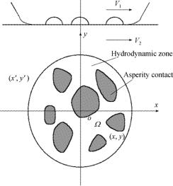
Fig. 1. Model of temperature calculation.
In this paper the temperature distribution of mixed lubrication in point contact is obtained by using the moving point heat source integration method. As a continuation of Hu and Zhu’s work this paper lays[14] the basis for further work on thermal mixed lubrication. A double linear interpolation function, similar to that for calculation of elastic deformation, is used in our analysis to calculate temperature integration, which gives a better accuracy than that of Qiu and Cheng[13]. Due to the symmetry of the enlarged coefficient matrix, the computational work can be reduced by 50% with a moving grid method[15]. Numerical samples validate the algorithm and program. The calculating results of the cases of smooth surface and

No. 4 |
SIMULATION OF TEMPERATURE DISTRIBUTION OF POINT CONTACTS |
367 |
isotropic sinusoidal surface are presented.
1Theoretical model
As shown in fig. 1, the Carstesian coordinate axes are fixed at the center of a computation domain. Two surfaces in contact move in the direction of x at velocities V1 and V2. Consider an
instantaneous point heat source of strength |
q(x ,y ,t )dx dy dt emitted at position (x ,y ) |
and |
|||
time t |
with no heat loss on the boundary. The heat fluxes assigned to two surfaces are |
[1 |
|||
f(x , y , t |
)]q (x , y , t ) and f(x , y , t |
) q (x , y , t |
), respectively, where |
+ + + |
de- |
f (x , y ,t ) |
|||||
notes a partition coefficient. The temperature rises on two surfaces at position (x,y) from time 0 to t can be thus expressed in non-dimensional form[5]
|
|
|
|
|
|
|
|
|
|
|
|
|
|
|
|
|
|
|
|
|
|
|
|
|
|
|
|
|
|
|
|
|
|
|
|
|
|
|
|
|
|
|
|
|
|
|
|
|
|
|
|
( |
|
|
, |
|
|
, |
|
|
|
|
|
|
|
|
|
|
|
|
|
|
|
|
|
|
|
|
|
|||
|
|
|
|
|
|
|
|
|
|
|
|
|
|
|
|
|
|
|
|
|
|
|
|
|
|
|
|
|
|
|
|
|
|
|
|
|
|
|
|
|
|
|
|
|
|
|
q |
x |
y |
t )d |
x |
d |
y |
d t |
|
|||||||||||||||||||||||||||
|
|
|
|
|
|
|
|
|
|
|
|
|
|
|
0 |
t |
|
|
|
|
|
|
|
|
|
|
|
|
|
|
|
|
|
|
|
|
|
|
|
|
|
|
|
|
||||||||||||||||||||||||||||||||||||||
|
|
|
|
|
|
|
|
|
|
|
|
|
|
|
|
|
|
|
|
|
|
|
|
|
|
|
|
|
|
|
|
|
|
|
|
|
|
|
|
|
||||||||||||||||||||||||||||||||||||||||||
|
|
|
|
|
|
|
|
|
|
|
|
|
|
|
|
|
|
|
|
|
|
|
|
|
|
|
|
|
|
|
|
|
|
|
|
|
|
|
|
|
||||||||||||||||||||||||||||||||||||||||||
T (x, y,t ) |
|
f (x , y ,t )] |
|
|
|
|
|
|
|
|
|
|
|
(t t )3/ 2 |
|
|
|
|
|
|
|
|
|
|
||||||||||||||||||||||||||||||||||||||||||||||||||||||||||
|
|
|
[1 |
|
|
|
|
|
|
|
|
|
|
|
|
|
|
|
|
|
|
|
|
|
|
|
|
|
|
|
|
|
|
|
|
|
|
|
|
|||||||||||||||||||||||||||||||||||||||||||
1 |
|
|
|
|
|
|
|
|
|
|
|
|
|
|
|
|
[( |
|
|
|
|
|
|
|
|
|
|
|
|
( |
|
|
|
|
|
t )]2 ( |
|
|
|
|
|
)2 |
|
|
|
|||||||||||||||||||||||||||||||||||||
|
|
|
|
|
|
|
|
|
|
|
|
|
|
|
|
|
|
|
|
|
|
|
|
|
|
|
|
|
|
|
|
|
|
|
|
|
|
|
||||||||||||||||||||||||||||||||||||||||||||
|
|
|
|
|
|
|
|
|
|
|
|
|
|
|
|
|
|
|
|
|
) V |
|
||||||||||||||||||||||||||||||||||||||||||||||||||||||||||||
|
|
|
|
|
|
|
|
|
|
|
|
|
|
|
|
|
|
x |
x |
t |
y |
y |
|
|||||||||||||||||||||||||||||||||||||||||||||||||||||||||||
|
|
|
|
|
|
|
|
|
|
|
|
|
|
|
|
|
|
|
|
|
|
1 |
|
|
|
|
|
|
|
|
|
|
|
|
|
|
|
|
|
|
|
|
|
|
|
|
|
|
|
|
|
|
|
|
|
|
|
|
|
|
|
|||||||||||||||||||||
|
|
|
|
|
|
|
|
|
|
|
|
|
|
|
exp |
|
|
|
|
|
|
|
|
|
|
|
|
|
|
|
|
|
|
|
|
|
|
|
|
|
|
|
|
|
|
|
|
|
|
|
|
|
|
|
|
|
|
|
|
|
|
|
|
|
|
|
|
|
, |
(1) |
||||||||||||
|
|
|
|
|
|
|
|
|
|
|
|
|
|
|
|
|
|
|
|
|
|
|
|
|
|
|
|
|
|
|
|
|
|
|
|
|
|
|
|
|
|
|
|
|
|
|
|
|
|
|
|
|
|
|
|
|
|
|
|
|
|
|
|
|
|
|
|
|||||||||||||||
|
|
|
|
|
|
|
|
|
|
|
|
|
|
|
|
|
|
|
|
|
|
|
|
|
|
|
|
|
|
|
|
|
|
|
|
|
(t t ) |
|
|
|
||||||||||||||||||||||||||||||||||||||||||
|
|
|
|
|
|
|
|
|
|
|
|
|
|
|
|
|
|
|
|
|
|
|
|
|
|
|
|
|
|
|
|
|
|
|
|
|
|
|
|
|
|
|
|
|
|
|
|
|
|
|
|
|
|
|
|
|
|
|
|
|
|
|
|
|
|
|
|
|
|
|
|
|
|
|
||||||||
|
|
|
|
|
|
|
|
|
|
|
|
|
|
|
|
|
|
|
|
|
|
|
|
|
|
|
|
|
|
|
|
|
|
|
|
|
|
|
|
|
( |
|
|
, |
|
|
, |
|
|
|
|
|
|
|
|
|
|
|
|
|
|
|
||||||||||||||||||||
|
|
|
|
|
|
|
|
|
|
|
|
|
|
|
|
|
|
|
|
|
|
|
|
|
|
|
|
|
|
|
|
|
|
|
|
q |
x |
y |
t )d |
x |
d |
y |
d t |
|
||||||||||||||||||||||||||||||||||||||
|
|
|
|
|
|
|
|
|
|
|
|
|
|
|
|
|
|
|
t |
|
|
|
|
|
|
|
|
|
|
|
|
|
|
|
|
|
|
|
||||||||||||||||||||||||||||||||||||||||||||
|
|
|
|
|
|
|
|
|
|
|
|
|
|
|
|
|
|
|
|
|
|
|
|
|
|
|
|
|
|
|
|
|
|
|
|
|
||||||||||||||||||||||||||||||||||||||||||||||
|
|
|
|
|
|
|
|
|
|
|
|
|
|
|
|
|
|
|
|
|
|
|
|
|
|
|
|
|
|
|
|
|
|
|
|
|
||||||||||||||||||||||||||||||||||||||||||||||
|
|
|
|
|
|
|
|
|
|
|
|
|
|
|
|
0 |
|
|
|
|
|
|
|
|
|
|
|
|
|
|
|
|
|
|
|
|
|
|
|
|
|
|
|
|
|
|
|
(t t )3/ 2 |
|
|
|
|
|
|
|
|
|
|
||||||||||||||||||||||||
T |
(x, y,t ) |
|
|
|
|
|
|
f (x , y ,t ) |
|
|
|
|
|
|
|
|
|
|
|
|
|
|
|
|
|
|
|
|
|
|
|
|
|
|
|
|
|
|
|
|
|
|
|
|
|
|
|
|
|
|
|
|
||||||||||||||||||||||||||||||
2 |
|
|
|
|
|
|
|
|
|
|
|
|
|
|
|
|
|
[( |
|
|
|
|
|
|
|
|
|
|
|
|
|
|
|
( |
|
|
|
|
|
t )]2 ( |
|
|
|
)2 |
|
|||||||||||||||||||||||||||||||||||||
|
|
|
|
|
|
|
|
|
|
|
|
|
|
|
|
|
|
|
|
|
|
|
|
|
|
|
|
|
|
|
|
|
||||||||||||||||||||||||||||||||||||||||||||||||||
|
|
|
|
|
|
|
|
|
|
|
|
|
|
|
|
|
|
|
|
|
|
|
) V |
|
||||||||||||||||||||||||||||||||||||||||||||||||||||||||||
|
|
|
|
|
|
|
|
|
|
|
|
|
|
|
|
|
|
|
|
|
x |
x |
t |
y |
y |
|
||||||||||||||||||||||||||||||||||||||||||||||||||||||||
|
|
|
|
|
|
|
|
|
|
|
|
|
|
|
|
|
|
|
|
|
|
|
|
|
|
|
|
|
|
|
|
|
|
|
|
|
|
|
2 |
|
|
|
|
|
|
|
|
|
|
|
|
|
|
|
|
|
|
|
|
|
|
|
|
|
|
|
|
|
|
|
|
|
|
|
|
|
||||||
|
|
|
|
|
|
|
|
|
|
|
|
|
|
|
|
exp |
|
|
|
|
|
|
|
|
|
|
|
|
|
|
|
|
|
|
|
|
|
|
|
|
|
|
|
|
|
|
|
|
|
|
|
|
|
|
|
|
|
|
|
|
|
|
|
|
|
|
|
|
|
|
|
. |
(2) |
|||||||||
|
|
|
|
|
|
|
|
|
|
|
|
|
|
|
|
|
|
|
|
|
|
|
|
|
|
|
|
|
|
|
|
|
|
|
|
|
|
|
|
|
|
|
|
|
|
|
|
|
|
|
|
|
|
|
|
|
|
|
|
|
|
|
|
|
|
|
|
|
|
|
||||||||||||
|
|
|
|
|
|
|
|
|
|
|
|
|
|
|
|
|
|
|
|
|
|
|
|
|
|
|
|
|
|
|
|
|
|
|
|
|
|
|
|
|
|
( |
t |
|
t ) |
|
|
|
|
|
|
|
||||||||||||||||||||||||||||||
|
|
|
|
|
|
|
|
|
|
|
|
|
|
|
|
|
|
|
|
|
|
|
|
|
|
|
|
|
|
|
|
|
|
|
|
|
|
|
|
|
|
|
|
|
|
|
|
|
|
|
|
|
|
|
|
|
|
|
|
|
|
|
|
|
|
|
|
|
|
|
|
|
|
|
|
|
|
|
||||
The heat flux density caused by friction can be expressed as |
|
|
|
|
|
|
|
|
|
|
||||||||||||||||||||||||||||||||||||||||||||||||||||||||||||||||||||||||
|
|
|
|
|
|
|
|
|
|
|
|
|
|
|
|
|
|
|
|
|
|
|
|
|
|
|
|
|
|
|
|
|
|
|
|
|
|
|
|
|
|
|
|
|
|
|
|
|
|
|
|
|
|
|
|
|
|
|
|
|
|
|
|
|
|
|
|
|
|
|
(3) |
|||||||||||
|
|
|
|
|
|
|
|
|
|
|
|
|
|
|
|
|
|
|
|
|
|
|
|
|
|
pVs. |
|
|
|
|
|
|
|
|
|
|
|
|
|
|
|
|
|
|
|
|
|
|
|
|
|
|
|
|
|
|
|
|
|
|
|
|
|
|
|
|
|
|
||||||||||||||
|
|
|
|
|
|
|
|
|
|
|
|
|
|
|
|
|
|
|
|
|
|
|
|
q |
|
|
|
|
|
|
|
|
|
|
|
|
|
|
|
|
|
|
|
|
|
|
|
|
|
|
|
|
|
|
|
|
|
|
|
|
|
|
|
|
|
|
||||||||||||||||
According to ref. [16], the friction coefficient has different values for different friction conditions of hydrodynamic lubrication, asperity contact and metal melting. The pressure in mixed lubrication is acquired with the program developed by Hu and Zhu[14]. The heat flux partition
coefficient |
|
|
+ |
|
+ |
|
+ |
|
is determined by the following condition of temperature equaling |
[16] |
||||||||||||||||||||||||||||||||||||||
|
|
|||||||||||||||||||||||||||||||||||||||||||||||
f (x , y ,t |
) |
: |
||||||||||||||||||||||||||||||||||||||||||||||
|
|
|
|
|
|
|
|
|
|
|
|
|
|
|
|
|
|
|
|
|
|
|
|
|
|
|
|
|
|
|
|
|
|
|
|
|
|
|
|
|
|
|
|
|
|
|
|
|
[T2b T2 ( |
|
, |
|
, |
|
)] [T1b T1( |
|
, |
|
, |
|
)] S [1 2 f ( |
|
, |
|
, |
|
|
)] h( |
|
, |
|
) |
|
( |
|
, |
|
, |
|
). |
(4) |
||||||||||||||||
x |
y |
t |
x |
y |
t |
x |
y |
t |
x |
y |
q |
x |
y |
t |
||||||||||||||||||||||||||||||||||
For asperity contact points the above equation is valid by setting |
|
( |
|
, |
|
) 0 . |
|
|||||||||||||||||||||||||||||||||||||||||
h |
|
|||||||||||||||||||||||||||||||||||||||||||||||
x |
y |
|
||||||||||||||||||||||||||||||||||||||||||||||
2Algorithm and program
The spatial domain is divided into M N element meshes, and time domain from 0 to t
is divided into P small time intervals. (1) (4) are discretized in the spatial and time domain. The discretized form of (1) is
|
|
|
|
|
|
|
|
P |
M |
N |
|
||
|
|
( |
|
, |
|
, |
|
|
|
e (i, j,k), |
(5) |
||
T1 |
|
|
|
) T1 |
|||||||||
x |
y |
t |
|||||||||||
|
|
|
|
|
|
|
|
k 1 |
i 1 |
j 1 |
|
||
where "T1 e (i, j,k) represents the integration on one element with respect to given (x, y,t ) .

368 SCIENCE IN CHINA (Series E) Vol. 45
|
|
|
|
|
|
|
|
|
|
|
|
|
|
|
|
|
|
|
|
|
|
|
|
|
|
|
|
|
( |
|
, |
|
, |
|
|
|
|
|
|
|
|
|
|
|
|||
|
|
|
|
|
|
|
|
|
|
|
|
|
|
|
|
|
|
|
q |
x |
y |
t )d |
x |
d |
y |
d t |
|||||||||||||||||||||
|
|
e |
|
|
tk |
xi |
|
|
|
y |
j |
|
|
|
|
|
|
|
|
|
|
|
|
|
|
|
|||||||||||||||||||||
|
|
|
|
|
|
|
|
|
|
|
|
|
|
|
|
|
|||||||||||||||||||||||||||||||
|
|
|
|
|
|
|
|
|
|
|
|
|
|
|
|
|
|||||||||||||||||||||||||||||||
T |
|
(i, j,k) |
|
|
|
|
|
|
|
|
|
|
|
[1 f (x , y ,t )] |
|
|
|
|
|
|
|
|
|
|
|
|
|
|
|
|
|
|
|
||||||||||||||
1 |
|
|
|
|
|
|
|
|
|
|
|
|
|
|
|
|
|
|
|
|
|
|
|
|
|
|
|
|
|
|
|
|
|
|
|
|
|
|
|
|
|
|
|
|
|
||
|
|
|
|
tk 1 |
xi 1 |
|
y |
j 1 |
|
|
|
|
|
|
(t t )3/ 2 |
||||||||||||||||||||||||||||||||
|
|
|
|
|
|
|
[( |
|
|
|
|
|
|
( |
|
|
|
|
t )]2 |
( |
|
|
|
)2 |
|||||||||||||||||||||||
|
|
|
|
|
|
|
|
|
|
) V |
|||||||||||||||||||||||||||||||||||||
|
|
|
|
|
|
x |
|
x |
t |
y |
y |
||||||||||||||||||||||||||||||||||||
|
|
|
|
|
|
|
|
|
|
|
|
|
1 |
|
|
|
|
|
|
|
|
|
|
|
|
|
|
|
|
|
|
|
|||||||||||||||
|
|
|
|
exp |
|
|
|
|
|
|
|
|
|
|
|
|
|
|
|
|
|
|
|
|
|
|
|
|
|
|
|
|
|
|
|
. |
|||||||||||
|
|
|
|
|
|
|
|
|
|
|
|
|
|
|
|
|
|
|
|
|
|
|
|
|
|
|
|
|
|
|
|
|
|
|
|||||||||||||
|
|
|
|
|
|
|
|
|
|
|
|
|
|
|
|
|
|
|
( |
t |
|
t ) |
|
|
|
|
|
|
|
|
|
|
|
|
|||||||||||||
|
|
|
|
|
|
|
|
|
|
|
|
|
|
|
|
|
|
|
|
|
|
|
|
|
|
|
|
|
|
|
|
|
|
|
|
|
|
|
|||||||||
Assume that the heat flux density and the heat partition function are invariant during one time interval. Similar to the calculation of elastic deformation, double linear interpolation func-
|
|
|
|
|
|
|
|
|
|
|
|
|
|
|
|
|
|
|
|
|
|
|
|
|
|
|
|
|
|
|
changes |
||||||
tions are used to describe the distribution of heat flux. The result shows that "T1 |
e (i, j,k) |
||||||||||||||||||||||||||||||||||||
into the sum of the integration at nodes of the element. |
|
|
|
|
|
||||||||||||||||||||||||||||||||
|
|
|
|
|
|
|
|
|
|
|
|
|
|
|
1 |
|
|
|
|
|
|
1 |
1 |
|
|
|
|
||||||||||
|
|
e |
|
|
|
|
|
|
|
|
|
|
|
|
|
|
|
t |
tk |
|
|
|
|
||||||||||||||
|
|
|
|
|
|
|
|
|
|
|
|
|
|
|
|
|
|||||||||||||||||||||
|
|
|
|
|
|
|
|
|
|
|
|
|
|
|
|
|
|||||||||||||||||||||
T1 |
(i, j,k) (1 f (l,h,k))q(l,h,k) |
|
|
|
|
|
|
|
|
|
|
|
|
|
|
|
gl,h du (l i 1,i;h j 1, |
j), (6) |
|||||||||||||||||||
|
|
x |
|
y |
u |
||||||||||||||||||||||||||||||||
t |
tk |
||||||||||||||||||||||||||||||||||||
where |
u t t + , |
gl,h |
is a function of positions and velocities. The integration in (6) has one |
||||||||||||||||||||||||||||||||||
singularity when |
tk t |
|
and can be eliminated by using an integration transform u e s . The |
||||||||||||||||||||||||||||||||||
|
|
|
|
|
|
|
|
|
|
|
|
|
is assembled with respect to node. Formula |
||||||||||||||||||||||||
overall temperature rise on all elements "T1 |
e (i, j,k) |
|
|
||||||||||||||||||||||||||||||||||
(5) becomes |
|
|
|
|
|
|
|
|
|
|
|
|
|
|
|
|
|
|
|
|
|
|
|
|
|
|
|
|
|
|
|
|
|
||||
|
|
|
|
|
|
|
|
|
|
|
|
|
P M |
N |
|
|
|
|
|
|
|
|
|
|
|
|
|
||||||||||
|
|
|
|
|
|
|
|
|
|
|
) [1 f (i, j,k)] |
|
|
|
|||||||||||||||||||||||
|
|
|
|
T1 |
( |
|
, |
|
, |
|
|
(i, j,k) C1(i, j,k), |
(7) |
||||||||||||||||||||||||
|
|
|
|
x |
y |
t |
q |
||||||||||||||||||||||||||||||
|
|
|
|
|
|
|
|
|
|
|
|
k 1 i 0 |
j 0 |
|
|
|
|
|
|
|
|
|
|
|
|
|
|||||||||||
where C1(i, j,k) is the influence coefficient representing the temperature rise at (x, y) , caused by a continuous unit point heat source emitted at (i, j) and in the time interval k.
With the same argument, one gets
|
|
|
|
|
|
|
|
P M |
N |
|
||||||
|
|
|
|
|
|
|
|
) f (i, j,k) |
|
|
|
|
|
|
|
|
T2 ( |
|
, |
|
, |
|
|
(i, j,k) C2 (i, j,k). |
(8) |
||||||||
x |
y |
t |
q |
|||||||||||||
|
|
|
|
|
|
|
|
k 1 i 0 |
j 0 |
|
||||||
From (7) we can see that the temperature rise at one point ( |
x |
, |
y |
) requires M N numeri- |
||||||||||||
cal integration operations, (M 1) (N 1) multiple operations and M N |
addition operations. |
|||||||||||||||
In order to raise efficiency, moving grid method[15] for calculating elastic deformation is applied. It requires an influence coefficient matrix of 2 (M 1) (N 1) , which means 2 (M 1) (N 1)
integration operations. It is found that the enlarged matrix is symmetric in the direction perpendicular to the velocity, so that the storage and computation of coefficient matrix can be reduced by 50%.
Substituting (7) and (8) into (4), we have the following discretized equation:
P M N |
|
q(i, j,k) { f (i, j,k) [C2 (i, j,k) C1(i, j,k)] C1(i, j,k)} |
|
k 1 i 0 j 0 |
|
(T1b T2b ) S [1 2 f (i, j,k)] h(i, j) q(i, j,k). |
(9) |
The heat partitions f (i, j,k) for different time intervals, obtained with (9) are substituted to into (7) and (8), which gives the temperature rises on two surfaces.

No. 4 |
SIMULATION OF TEMPERATURE DISTRIBUTION OF POINT CONTACTS |
369 |
3Validation
To verify the numerical scheme established in the previous sections, two numerical examples are presented here. The first numerical example is a uniform square heat source moving on a semi-infinite body. The dimensions of the square heat source are 2a 2a in x and y direc-
tion, respectively. Fig.2 shows a comparison of the present calculation with the results of Carslaw and Jaeger[5] and Tian and Kennedy[11] under the same condition of Pe 18.8 . The comparison,
which is made along the centerline in the sliding direction, indicates that the present approach yields a result in a good agreement with the methods in literature.
Another numerical example is given in fig. 3 for further comparison with existing work[9 11,13,17]. The contact geometry is the same as that of ref. [13]. The present approach again shows a close agreement with other existing methods, especially that of Francis[10].
Fig. 2. A comparison of present analysis with existing results.
Fig. 3. Comparison of maximum temperature.
4Results
The following two cases provide the simulation results of temperature distribution in point contacts. The contact conditions listed in the following are the same as those in ref. [14]. The Hertzian contact radius is a 0.4725 mm and the maximum Hertzian contact pressure is
ph 1.711GPa. The solution domain is determined as –1.9 x 1.1 and –1.5 y 1.5. The computational grid covering the domain consists of equally spaced 129×129 nodes. Material properties presented in ref. [13] are also used in this study. The specific heat and density of solids
are |
c 460 J/(kg·K) and |
7850 kg/m3. The thermal conductivities for solid and liquid are |
Ks |
48 W/(m·K) and Kf |
0.131 W/(m·K). Friction coefficients, , are 0.06, 0.10 and 0.40, |
corresponding to fluid lubrication, dry contact and metal melting respectively. The bulk temperatures are T1b T2b 0 K. In the calculations, the heat flux density is assumed to be constant in each time step. The results given in the following are the solutions for a steady state after the moving body passes through a distance 4 times Hertzian contact radius with given sliding velocity.
In the first case, smooth surfaces slide with velocities V1 2.5 and V2 7.5 m/s. The
370 |
SCIENCE IN CHINA (Series E) |
Vol. 45 |
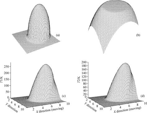
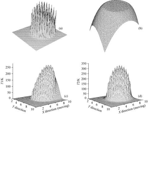
second case is designed for isotropic sinusoidal surfaces in sliding contact, with one surface moving at velocity V1 5 m/s and other surface stationary. The profiles of pressure, film thickness and temperature for the two cases are given in figs. 4 and 5. Fig. 6 gives a comparison of the results along the centerline in moving direction for the two cases. From these figures the following conclusions can be drawn:
(1)The shape of temperature rise looks like that of pressure since the inputting condition of heat flux is in direct proportion to pressure. However, due to the influence of velocity, higher temperature is observed in the outlet area.
(2)The maximum temperature rise on the surface with small velocity is higher than that on the surface with large velocity. The reason is that the relative moving velocity of heat source is low at the slow moving surface so that the effects of heat accumulation are significant, which gives higher temperature rise.
(3)As shown in fig. 6(b), the interactive influence of temperature is stronger than that of the pressure.
Fig. 4. The case of smooth surfaces. (a) Pressure distribution; (b) film thickness distribution; (c) temperature distribution of
surface 1; (d) temperature distribution of surface 2.
5Conclusion
A model for evaluation of the transient temperature distribution in point contact of mixed lubrication is presented. Due to the symmetry of enlarged influence coefficient matrix in the direc-
No. 4 |
SIMULATION OF TEMPERATURE DISTRIBUTION OF POINT CONTACTS |
371 |
Fig. 5. The case of isotropic sinusoidal surfaces. (a) Pressure distribution; (b) film thickness distribution; (c) temperature distribution of surface 1; (d) temperature distribution of surface 2.
Fig. 6. Results along centerline in X direction. (a) The case of smooth surfaces; (b) the case of isotropic sinusoidal surfaces.
tion perpendicular to the velocity, the storage and computational work are further reduced by 50%. Numerical samples of a uniform square heat source and parabolic heat source validate the algorithm and program. The calculating results on the smooth and isotropic sinusoidal surfaces in point contacts are presented, with which the influence of velocities, heat accumulation and heat interaction has been discussed.
References
1.Tian Xuefeng, Kennedy, F. E., Contact surface temperature models for finite bodies in dry and boundary lubricated sliding, ASME, Journal of Tribology, 1993, 115(3): 411.
2.Zhu Dong, Wen Shizhu, A full numerical solution for the thermoelastohydrodynamic problem in elliptical contacts, ASME,

372 SCIENCE IN CHINA (Series E) Vol. 45
Journal of Tribology, 1984, 106(2): 246.
3. Vilmos, S., Thermal elastohydrodynamic lubrication of rider rings, ASME, Journal of Tribology, 1984, 106(4): 492 498.
4.Guo Feng, Yang Peiran, Influence of a ring flat zone in the point contact surface in thermal elastohydyodynamic lubrication, Tribology International, 1999, 32: 167.
5. Carslaw, H. S., Jeager, J. C., Conduction of Heat in Solids, 2nd ed, London: Oxford Press, 1959, 266 270.
6.Bruggemann, H., Kollmann, F. G., A numerical solution of the thermal elastohydrodynamic lubrication in an elliptical contact, ASME, Journal of Tribology, 1982, 104(3): 392.
7.Ghosh, M. K., Harmrock, B. J., Thermal elastohydrodynamic lubrication of line contacts, ASLE Transaction, 1984, 28(2): 159.
8.Zhu, D., Cheng, H. S., An analysis and computational procedure for EHL film thickness, friction and flash temperature in line and point contacts, Tribology Transaction, 1989, 32(3): 364.
9.Blok, H., Theoretical study of temperature rise at surfaces of actual contact under oiliness conditions, Proc. General discussion on lubrication, London: Inst. Mech. Engrs., 1937, 14: 222.
10.Francis, H. A., Interfacial temperature distribution within a sliding Hertzian contact, ASLE Transaction, 1970, 14(1): 41.
11.Tian Xuefeng, Kennedy, F. E., Maximum and average flash temperature in sliding contacts, ASME, Journal of Tribology, 1994, 116: 167.
12.Zhai Xuejun, Chang, L., A transient thermal model for mixed-film contacts, Tribology Transaction, 2000, 43(3): 427.
13.Qiu, Liangheng, Cheng, H. S., Temperature rise simulation of three-dimensional rough surface in mixed lubricated contact, ASME, Journal of Tribology, 1998, 120(2): 310.
14.HuYuanzhong, Zhu Dong, A full numerical solution to the mixed lubrication in point contact, Tribology Transaction, 2000, 44(1): 1.
15.Ren Ning, Lee, S. C., Contact simulation of three dimensional rough surfaces using moving grid method, ASME, Journal of Tribology, 1993, 115(4): 597.
16.Lai, W. T., Cheng, H. S., Temperature analysis in lubricated simple sliding rough contacts, ASLE Transaction, 1984, 128(3): 302.
17.Gao, Jianjun, Lee, S. C., Ai Xiaolan et al., An FFT-based transient flash temperature model of general three-dimensional rough surface contacts, ASME, Journal of Tribology, 2000, 122(3): 519.