lab-inf-4_tasks / 2000_34

1

The sixth section describes work on the common phenomenon of stick-slip motion, and microscopic models for its origins. Atomic-scale ratcheting is contrasted with long-range slip events, and the structural changes that accompany stick-slip transitions in simulations are described.

The seventh and final section describes work on friction at extreme conditions such as high shear rates or large contact pressures. Simulations of tribochemical reactions, machining, and the evolution of microstructure in sliding contacts are discussed.

II. ATOMISTIC COMPUTER SIMULATIONS

The simulations described in this chapter all use an approach called classical molecular dynamics (MD) that is described extensively in a number of review articles and books, including Allen and Tildesley (1987) and Frenkel and Smit (1996). The basic outline of the method is straightforward. One begins by defining the interaction potentials. These produce forces on the individual particles whose dynamics will be followed, typically atoms or molecules. Next the geometry and boundary conditions are specified, and initial coordinates and velocities are given to each particle. Then the equations of motion for the particles are integrated numerically, stepping forward in time by discrete steps of size t. Quantities such as forces, velocities, work, heat flow, and correlation functions are calculated as a function of time to determine their steady-state values and dynamic fluctuations. The relation between changes in these quantities and the motion of individual molecules is also explored.

When designing a simulation, care must be taken to choose interaction potentials and ensembles that capture the essential physics that is to be addressed. The potentials may be as simple as ideal spring constants for studies of general phenomena, or as complex as electronic density-functional calculations in quantitative simulations. The ensemble can also be tailored to the problem of interest. Solving Newton’s equations yields a constant energy and volume, or microcanonical, ensemble. By adding terms in the equation of motion that simulate heat baths or pistons, simulations can be done at constant temperature, pressure, lateral force, or velocity. Constant chemical potential can also be maintained by adding or removing particles using Monte Carlo methods or explicit particle baths.

The amount of computational e ort typically grows linearly with both the number of particles, N , and the number of time-steps M . The prefactor increases rapidly with the complexity of the interactions, and substantial ingenuity is required to achieve linear scaling with N for long-range interactions or density-functional approaches. Complex interactions also lead to a wide range of characteristic frequencies, such as fast bond-stretching and slow bond-bending modes. Unfortunately, the time step t must be small ( 2%) compared to the period of the fastest mode. This means that many time steps are needed before one obtains information about the slow modes.

The maximum feasible simulation size has increased continuously with advances in computer technology, but remains relatively limited. The product of N times M in the largest simulations described below is about 1012. A cubic region of 106 atoms would have a side of about 50nm. Such linear dimensions allow reasonable models of an atomic force microscope tip, the boundary lubricant in a surface force apparatus, or an individual asperity contact on a rough surface. However 106 time steps is only about 10 nanoseconds, which is much smaller than experimental measurement times. This requires intelligent choices in the problems that are attacked, and how results are extrapolated to experiment. It also limits sliding velocities to relatively high values, typically meters per second or above.

A number of e orts are underway to increase the accessible time scale, but the problem remains unsolved. Current algorithms attempt to follow the deterministic equations of motion, usually with the Verlet or predictor-corrector algorithms (Allen and Tildesley, 1987). One alternative approach is to make stochastic steps. This would be a non-equilibrium generalization of the Monte Carlo approach that is commonly used in equilibrium systems. The di culty is that there is no general principle for determining the appropriate probability distribution of steps in a non-equilibrium system.

In the following we describe some of the potentials that are commonly used, and the situations where they are appropriate. The final two subsections describe methods for maintaining constant temperature and constant load.

A. Model Potentials

A wide range of potentials has been employed in studies of tribology. Many of the studies described in the next section use simple ideal springs and sine-wave potentials. The Lennard-Jones potential gives a more realistic representation of typical inter-atomic interactions, and is also commonly used in studies of general behavior. In order to model specific materials, more detail must be built into the potential. Simulations of metals frequently use the embedded atom method, while studies of hydrocarbons use potentials that include bond-stretching, bending, torsional

2

forces and even chemical reactivity. In this section we give a brief definition of the most commonly used models. The reader may consult the original literature for more detail.

The Lennard-Jones (LJ) potential is a two-body potential that is commonly used for interactions between atoms or molecules with closed electron shells. It is applied not only to the interaction between noble gases, but also to the interaction between di erent segments on polymers. In the latter case, one LJ particle may reflect a single atom on the chain (explicit atom model), a CH2 segment (united atom model) or even a Kuhn’s segment consisting of several CH2 units (coarse-grained model). United atom models (Ryckaert and Bellemans, 1978) have been shown by Paul et al. (1995) to successfully reproduce explicit atom results for polymer melts, while Tsch¨op et al. (1998a, 1998b) have successfully mapped chemically detailed models of polymers onto coarse-grained models and back.

The 12-6 LJ potential has the form

where rij is the distance between particles i and j, ǫ is the LJ interaction energy, and σ is the LJ interaction radius. The exponents 12 and 6 used above are very common, but depending on the system, other values may be chosen. Many of the simulation results discussed in subsequent sections are expressed in units derived from ǫ, σ, and a

pressures and temperatures that are not too large.

Most realistic atomic potentials can not be expressed as two-body potentials. For example, bond angle potentials in a polymer are e ectively three-body interactions and torsional potentials correspond to four-body interactions. Classical models of these interactions (Flory, 1988; Binder, 1995) assume that a polymer is chemically inert and interactions between di erent molecules are modeled by two-body potentials. In the most sophisticated models, bond-stretching, bending and torsional energies depend on the position of neighboring molecules and bonds are allowed to rearrange (Brenner, 1990). Such generalized model potentials are needed to model friction-induced chemical interactions.

For the interaction between metals, a di erent approach has proven fruitful. The embedded atom method (EAM), introduced by Daw and Baskes (1984), includes a contribution in the potential energy associated with the cost of ”embedding” an atom in the local electron density ρi produced by surrounding atoms. The total potential energy U

˜

where Fi is the embedding energy, whose functional form depends on the particular metal. The pair potential φij (rij ) is a doubly-screened short-range potential reflecting core-core repulsion. The computational cost of the EAM is not substantially greater than pair potential calculations because the density ρi is approximated by a sum of independent atomic densities. When compared to simple two-body potentials such as Lennard-Jones or Morse potentials, the EAM has been particularly successful in reproducing experimental vacancy formation energies and surface energies, even though the potential parameters were only adjusted to reproduce bulk properties. This feature makes the EAM an important tool in tribological applications, where surfaces and defects play a major role.

B. Maintaining Constant Temperature

An important issue for tribological simulations is temperature regulation. The work done when two walls slide past each other is ultimately converted into random thermal motion. The temperature of the system would increase indefinitely if there was no way for this heat to flow out of the system. In an experiment, heat flows away from the sliding interface into the surrounding solid. In simulations, the e ect of the surrounding solid must be mimicked by coupling the particles to a heat bath.

Techniques for maintaining constant temperature T in equilibrium systems are well-developed. Equipartition guarantees that the average kinetic energy of each particle along each Cartesian coordinate is kB T /2 where kB is Boltzmann’s constant. To thermostat the system, the equations of motion are modified so that the average kinetic energy stays at this equilibrium value.

This assumes that T is above the Debye temperature so that quantum statistics are not important. The applicability of classical MD decreases at lower T .

3

One class of approaches removes or adds kinetic energy to the system by multiplying the velocities of all particles by the same global factor. In the simplest version, velocity rescaling, the factor is chosen to keep the kinetic energy exactly constant at each time step. However, in a true constant temperature ensemble there would be fluctuations in the kinetic energy. Improvements, such as the Berendsen and Nos´e-Hoover methods (Nos´e, 1991) add equations of motion that gradually scale the velocities to maintain the correct average kinetic energy over a longer time scale.

Another approach is to couple each atom to its own local thermostat (Schneider and Stoll, 1978; Grest and Kremer, 1986). The exchange of energy with the outside world is modeled by a Langevin equation that includes a damping

~

coe cient γ and a random force fi(t) on each atom i. The equations of motion for the α component of the position xiα become:

where U is the total potential energy and mi is the mass of the atom. To produce the appropriate temperature, the forces must be completely random, have zero mean, and have a second moment given by

The damping coe cient γ must be large enough that energy can be removed from the atoms without substantial temperature increases. However, it should be small enough that the trajectories of individual particles are not perturbed too strongly.

The first issue in non-equilibrium simulations is what temperature means. Near equilibrium, hydrodynamic theories define a local temperature in terms of the equilibrium equipartition formula and the kinetic energy relative to the local rest frame (Sarman et al., 1998). In d dimensions, the definition is

where the sum is over all N particles and h~v(~x)i is the mean velocity in a region around ~x. As long as the change in mean velocity is su ciently slow, h~v(~x)i is well-defined, and this definition of temperature is on solid theoretical ground.

When the mean velocity di erence between neighboring molecules becomes comparable to the random thermal velocities, temperature is not well-defined. An important consequence is that di erent strategies for defining and controlling temperature give very di erent structural order and friction forces (Evans and Morriss, 1986; Loose and Ciccotti, 1992; Stevens and Robbins, 1993). In addition, the distribution of velocities may become non-Gaussian, and di erent directions α may have di erent e ective temperatures. Care should be taken in drawing conclusions from simulations in this extreme regime. Fortunately, the above condition typically implies that the velocities of neighboring atoms di er by something approaching 10% of the speed of sound. This is generally higher than any experimental velocity, and would certainly lead to heat buildup and melting at the interface.

In order to mimic experiments, the thermostat is often applied only to those atoms that are at the outer boundary of the simulation cell. This models the flow of heat into surrounding material that is not included explicitly in the simulation. The resulting temperature profile is peaked at the shearing interface (e.g. Bowden and Tabor, 1986; Khare et al., 1996). In some cases the temperature rise may lead to undesirable changes in the structure and dynamics even at the lowest velocity that can be treated in the available simulation time. In this case, a weak thermostat applied throughout the system may maintain the correct temperature and yield the dynamics that would be observed in longer simulations at lower velocities. The safest course is to couple the thermostat only to those velocity components that are perpendicular to the mean flow. This issue is discussed further in Sec. III E.

There may be a marginal advantage to local Langevin methods in non-equilibrium simulations because they remove heat only from atoms that are too hot. Global methods like Nos´e-Hoover remove heat everywhere. This can leave high temperatures in the region where heat is generated, while other regions are at an artificially low temperature.

C. Imposing Load and Shear

The magnitude of the friction that is measured in an experiment or simulation may be strongly influenced by the way in which the normal load and tangential motion are imposed (Rabinowicz, 1965). Experiments almost always impose a constant normal load. The mechanical system applying shear can usually be described as a spring attached to a stage moving at controlled velocity. The e ective spring constant includes the compliance of all elements of the

4

loading device, including the material on either side of the interface. Very compliant springs apply a nearly constant force, while very sti springs apply a nearly constant velocity.

In simulations, it is easiest to treat the boundary of the system as rigid, and to translate atoms in this region at a constant height and tangential velocity. However this does not allow atoms to move around (Sec. III D) or up and over atoms on the opposing surface. Even the atomic-scale roughness of a crystalline surface can lead to order of magnitude variations in normal and tangential force with lateral position when sliding is imposed in this way (Harrison et al., 1992b, 1993; Robbins and Baljon, 2000). The di erence between constant separation and pressure simulations of thin films can be arbitrarily large, since they produce di erent power law relations between viscosity and sliding velocity (Sec. V B).

One way of minimizing the di erence between constant separation and pressure ensembles is to include a large portion of the elastic solids that bound the interface. This extra compliance allows the surfaces to slide at a more uniform normal and lateral force. However, the extra atoms greatly increase the computational e ort.

To simulate the usual experimental ensemble more directly, one can add equations of motion that describe the position of the boundary (Thompson et al., 1990b, 1992, 1995), much as equations are added to maintain constant temperature. The boundary is given an e ective mass that moves in response to the net force from interactions with mobile atoms and from the external pressure and lateral spring. The mass of the wall should be large enough that its dynamics are slower than those of individual atoms, but not too much slower, or the response time will be long compared to the simulation time. The spring constant should also be chosen to produce an appropriate response time and ensemble.

III.WEARLESS FRICTION IN LOW DIMENSIONAL SYSTEMS

A. Two Simple Models of Crystalline Surfaces in Direct Contact

Static and kinetic friction involve di erent aspects of the interaction between surfaces. The existence of static friction implies that the surfaces become trapped in a local potential energy minimum. When the bottom surface is held fixed, and an external force is applied to the top surface, the system moves away from the minimum until the derivative of the potential energy balances the external force. The static friction Fs is the maximum force the potential can resist, i.e. the maximum slope of the potential. When this force is exceeded, the system begins to slide, and kinetic friction comes in to play. The kinetic friction Fk (v) is the force required to maintain sliding at a given velocity v. The rate at which work is done on the system is v · Fk (v) and this work must be dissipated as heat that flows away from the interface. Thus simulations must focus on the nature of potential energy minima to probe the origins of static friction, and must also address dissipation mechanisms to understand kinetic friction.

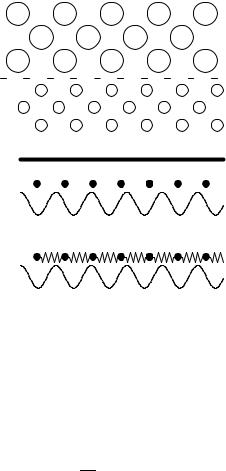
Two simple ball and spring models are useful in illustrating the origins of static and kinetic friction, and in understanding the results of detailed simulations. Both consider two clean, flat, crystalline surfaces in direct contact (Fig. 1a). The bottom solid is assumed to be rigid, so that it can be treated as a fixed periodic substrate potential acting on the top solid. In order to make the problem analytically tractable, only the bottom layer of atoms from the top solid is retained, and the interactions within the top wall are simplified. In the Tomlinson model (Fig. 1b), the atoms are coupled to the center of mass of the top wall by springs of sti ness k, and coupling between neighboring atoms is ignored (Tomlinson, 1929; McClelland and Cohen, 1990). In the Frenkel-Kontorova model (Fig. 1c), the atoms are coupled to nearest-neighbors by springs, and the coupling to the atoms above is ignored (Frenkel and Kontorova, 1938). Due to their simplicity, these models arise in a number of di erent problems and a great deal is known about their properties. McClelland (1989) and McClelland and Glosli (1992) have provided two early discussions of their relevance to friction. Bak (1982) has reviewed the Frenkel-Kontorova model and the physical systems that it models in di erent dimensions.

B. Metastability and Static Friction in One Dimension

Many features of the Tomlinson and Frenkel-Kontorova models can be understood from their one-dimensional versions. One important parameter is the ratio η between the lattice constants of the two surfaces η ≡ b/a. The other is the strength of the periodic potential from the substrate relative to the spring sti ness k that represents interactions within the top solid. If the substrate potential has a single Fourier component, then the periodic force can be written as

5

(a)

k

(b)

k

(c)

FIG. 1. (a) Two ideal, flat crystals making contact at the plane indicated by the dashed line. The nearest-neighbor spacings in the bottom and top walls are a and b respectively. The Tomlinson model (b) and Frenkel-Kontorova model (c) replace the bottom surface by a periodic potential. The former model keeps elastic forces between atoms on the top surface and the center of mass of the top wall, and the latter includes springs of sti ness k between neighbors in the top wall. (From Robbins, 2000.)

The relative strength of the potential and springs can be characterized by the dimensionless constant λ ≡ 2πf1/ka. In the limit of infinitely strong springs (λ → 0), both models represent rigid solids. The atoms of the top wall

are confined to lattice sites x0l = xCM + lb, where the integer l labels successive atoms, and xCM represents a rigid translation of the entire wall. The total lateral or friction force is given by summing Eq. 3.1

where N is the number of atoms in the top wall. In the special case of equal lattice constants (η = b/a = 1), the forces on all atoms add in phase, and F = −N f1 sin(2πxCM/a). The maximum of this restraining force gives the static friction Fs = N f1.

Unless there is a special reason for b and a to be related, η is most likely to be an irrational number. Such surfaces are called incommensurate, while surfaces with a rational value of η are commensurate. When η is irrational, atoms on the top surface sample all phases of the periodic force with equal probability and the net force (Eq. 3.2) vanishes exactly.

When η is a rational number, it can be expressed as p/q where p and q are integers with no common factors. In this case, atoms only sample q di erent phases. The net force from Eq. 3.2 still vanishes because the force is a pure sine wave and the phases are equally spaced. However, the static friction is finite if the potential has higher harmonics. A Fourier component with wavevector q2π/a and magnitude fq contributes N fq to Fs. Studies of surface potentials (Bruch et al., 1997) show that fq drops exponentially with increasing q and thus imply that Fs will only be significant for small q.

As the springs become weaker, the top wall is more able to deform into a configuration that lowers the potential energy. The Tomlinson model is the simplest case to consider, because each atom can be treated as an independent oscillator within the upper surface. The equations of motion for the position xl of the lth atom can be written as

6

FIG. 2. Graphical solution for metastability of an atom in the Tomlinson model for (a) λ = 0.5 and (b) λ = 3. The straight dashed lines show the force from the spring, k(xL − x0L ), at di erent x0L , and the curved lines show the periodic substrate potential. For λ < 1 there is a single intersection of the dashed lines with the substrate potential for each value of x0L , and thus a single metastable state. For λ > 1 there are multiple intersections with the substrate potential. Dotted portions of the potential curve indicate unstable maxima and solid regions indicate metastable solutions. As x0L increases, an atom that started at xL = 0 gradually moves through the set of metastable states indicated by a thick solid line. At the value of x0L corresponding to the third dashed line, this metastable state becomes unstable and the atom jumps to the metastable state indicated by the continuation of the thick region of the line. It then follows this portion of the line until this state becomes unstable at the x0L corresponding to the rightmost dashed line.

where m is the atomic mass and x0l is the position of the lattice site. Here γ is a phenomenological damping coe cient, like that in a Langevin thermostat (Sec. II B), that allows work done on the atom to be dissipated as heat. It represents the coupling to external degrees of freedom such as lattice vibrations in the solids.

In any steady-state of the system, the total friction can be determined either from the sum of the forces exerted by the springs on the top wall, or from the sum of the periodic potentials acting on the atoms (Eq. 3.2). If the time average of these forces di ered, there would be a net force on the atoms and a steady acceleration (Thompson and Robbins, 1990a; Matsukawa and Fukuyama, 1994). The static friction is related to the force in metastable states of

As shown graphically in Fig. 2a, there is only one solution for weak interfacial potentials and sti solids (λ < 1). In this limit, the behavior is essentially the same as for infinitely rigid solids. There is static friction for η = 1, but not for incommensurate cases. Even though incommensurate potentials displace atoms from lattice sites, there are exactly as many displaced to the right as to the left, and the force sums to zero.

A new type of behavior sets in when λ exceeds unity. The interfacial potential is now strong enough compared to the springs that multiple metastable states are possible. These states must satisfy both Eq. 3.4 and the condition that the second derivative of the potential energy is positive: 1 + λ cos (2πxl/a) > 0. The number of metastable solutions increases as λ increases.

As illustrated in Fig. 2b, once an atom is in a given metastable minimum it is trapped there until the center of mass moves far enough away that the second derivative of the potential vanishes and the minimum becomes unstable. The atom then pops forward very rapidly to the nearest remaining metastable state. This metastability makes it possible to have a finite static friction even when the surfaces are incommensurate.

If the wall is pulled to the right by an external force, the atoms will only sample the metastable states corresponding to the thick solid portion of the substrate potential in Fig. 2b. Atoms bypass other portions as they hop to the adjacent metastable state. The average over the solid portion of the curve is clearly negative and thus resists the external force. As λ increases, the dashed lines in Fig. 2b become flatter and the solid portion of the curve becomes confined to more and more negative forces. This increases the static friction which approaches N f1 in the limit λ → ∞ (Fisher, 1985).

7

A similar analysis can be done for the one-dimensional Frenkel-Kontorova model (Frank et al., 1949; Bak, 1982; Aubry, 1979, 1983). The main di erence is that the static friction and ground state depend strongly on η. For any given irrational value of η there is a threshold potential strength λc . For weaker potentials, the static friction vanishes. For stronger potentials, metastability produces a finite static friction. The transition to the onset of static friction was termed a breaking of analyticity by Aubry (1979) and is often called the Aubry transition. The metastable states for λ > λc take the form of locally commensurate regions that are separated by domain walls where the two crystals are out of phase. Within the locally commensurate regions the ratio of the periods is a rational number p/q that is close to η. The range of η where locking occurs grows with increasing potential strength (λ) until it spans all values. At this point there is an infinite number of di erent metastable ground states that form a fascinating “Devil’s staircase” as η varies (Aubry, 1979, 1983; Bak, 1982).

Weiss and Elmer (1996) have performed a careful study of the 1D Frenkel-Kontorova-Tomlinson model where both types of springs are included. Their work illustrates how one can have a finite static friction at all rational η and an Aubry at all irrational η. They showed that magnitude of the static friction is a monotonically increasing function of λ and decreases with decreasing commensurability. If η = p/q then the static friction rises with corrugation only as λq . Successive approximations to an irrational number involve progressively larger values of q. Since λc < 1, the value of Fs at λ < λc drops closer and closer to zero as the irrational number is approached. At the same time, the value of Fs rises more and more rapidly with λ above λc . In the limit q → ∞ one has the discontinuous rise from zero to finite values of Fs described by Aubry. Weiss and Elmer also considered the connection between the onsets of static friction, of metastability, and of a finite kinetic friction as v → 0 that is discussed in the next section. Their numerical results showed that all these transitions coincide.

Work by Kawaguchi and Matsukawa (1998) shows that varying the strengths of competing elastic interactions can lead to even more complex friction transitions. They considered a model proposed by Matsukawa and Fukuyama (1994) that is similar to the one-dimensional Frenkel-Kontorova-Tomlinson model. For some parameters the static friction oscillated several times between zero and finite values as the interaction between surfaces increased. Clearly the transitions from finite to vanishing static friction continue to pose a rich mathematical challenge.

C. Metastability and Kinetic Friction

The metastability that produces static friction in these simple models is also important in determining the kinetic friction. The kinetic friction between two solids is usually fairly constant at low center of mass velocity di erences vCM. This means that the same amount of work must be done to advance by a lattice constant no matter how slowly the system moves. If the motion were adiabatic, this irreversible work would vanish as the displacement was carried out more and more slowly. Since it does not vanish, some atoms must remain very far from equilibrium even in the

limit vCM → 0.

The origin of this non-adiabaticity is most easily illustrated with the Tomlinson model. In the low velocity limit, atoms stay near to the metastable solutions shown in Fig. 2. For λ < 1 there is a unique metastable solution that evolves continuously. The atoms can move adiabatically, and the kinetic friction vanishes as vCM → 0. For λ > 1 each atom is trapped in a metastable state. As the wall moves, this state becomes unstable and the atom pops rapidly to the next metastable state. During this motion the atom experiences very large forces and accelerates to a peak velocity vp that is independent of vCM. The value of vp is typically comparable to the sound and thermal velocities in the solid and thus can not be treated as a small perturbation from equilibrium. Periodic pops of this type are seen in many of the realistic simulations described in Sec. IV. They are frequently referred to as atomic-scale stick-slip motion (Secs. IV B and VI), because of the oscillation between slow and rapid motion (Sec. VI).

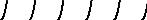
The dynamic equation of motion for the Tomlinson model (Eq. 3.3) has been solved in several di erent contexts. It is mathematically identical to simple models for Josephson junctions (McCumber, 1968), to the single-particle model of charge-density wave depinning (Gr¨uner et al., 1981), and to the equations of motion for a contact line on a periodic surface (Raphael and deGennes, 1989; Joanny and Robbins, 1990). Fig. 3 shows the time-averaged force as a function of wall velocity for several values of the interface potential strength in the overdamped limit. (Since each atom acts as an independent oscillator, these curves are independent of η.) When the potential is much weaker than the springs (λ < 1), the atoms can not deviate significantly from their equilibrium positions. They go up and down over the periodic potential at constant velocity in an adiabatic manner. In the limit vCM → 0 the periodic potential is sampled uniformly and the kinetic friction vanishes, just as the static friction did for incommensurate walls. At finite velocity the kinetic friction is just due to the drag force on each atom and rises linearly with velocity. The same result holds for all spring constants in the Frenkel-Kontorova model with equal lattice constants (η = 1).

As the potential becomes stronger, the periodic force begins to contribute to the kinetic friction of the Tomlinson model. There is a transition at λ = 1, and at larger λ the kinetic friction remains finite in the limit of zero velocity.

8

FIG. 3. Force vs. velocity for the Tomlinson model at the indicated values of λ. The force is normalized by the static friction N f1 and the velocity is normalized by v0 ≡ f1/γ where γ is the phenomenological damping rate. (Data from Joanny and Robbins, 1990).

The limiting Fk (v = 0) is exactly equal to the static friction for incommensurate walls. The reason is that as vCM → 0 atoms spend almost all of their time in metastable states. During slow sliding, each atom samples all the metastable states that contribute to the static friction and with exactly the same weighting.

The solution for commensurate walls has two di erent features. The first is that the static friction is higher than Fk (0). This di erence is greatest for the case λ < 1 where the kinetic friction vanishes, while the static friction is finite. The second di erence is that the force/velocity curve depends on whether the simulation is done at constant wall velocity (Fig. 3) or constant force. The constant force solution is independent of λ and equals the constant velocity solution in the limit λ → ∞.

The only mechanism of dissipation in the Tomlinson model is through the phenomenological damping force, which is proportional to the velocity of the atom. The velocity is essentially zero except in the rapid pops that occur as a state becomes unstable and the atom pops to the next metastable state. In the overdamped limit, atoms pop with peak velocity vp f1/γ – independent of the average velocity of the center of mass. Moreover, the time of the pop is nearly independent of vCM, and so the total energy dissipated per pop is independent of vCM. This dissipated energy is of course consistent with the limiting force determined from arguments based on the sampling of metastable states given above (Fisher, 1985; Raphael and DeGennes, 1989; Joanny and Robbins, 1990). The basic idea that kinetic friction is due to dissipation during pops that remain rapid as vCM → 0 is very general, although the phenomenological damping used in the model is far from realistic. A constant dissipation during each displacement by a lattice constant immediately implies a velocity independent Fk , and vice versa.

D. Tomlinson Model in Two-Dimensions: Atomic Force Microscopy

Gyalog et al. (1995) have studied a generalization of the Tomlinson model where the atoms can move in two dimensions over a substrate potential. Their goal was to model the motion of an atomic-force microscope (AFM) tip over a surface. In this case the spring constant k reflects the elasticity of the cantilever, the tip, and the substrate. It will in general be di erent along the scanning direction than along the perpendicular direction.

The extra degree of freedom provided by the second dimension means that the tip will not follow the nominal scanning direction, but will be deflected to areas of lower potential energy. This distorts the image and also lowers the measured friction force. The magnitude of both e ects decreases with increasing sti ness.

As in the one-dimensional model there is a transition from smooth sliding to rapid jumps with decreasing spring sti ness. However, the transition point now depends on sliding direction and on the position of the scan line along the direction normal to the nominal scan direction. Rapid jumps tend to occur first near the peaks of the potential, and

9

extend over greater distances as the springs soften. The curves defining the unstable points can have very complex, anisotropic shapes.

H¨olscher et al. (1997) have used a similar model to simulate scans of MoS2. Their model also includes kinetic and damping terms in order to treat the velocity dependence of the AFM image. They find marked anisotropy in the friction as a function of sliding direction, and also discuss deviations from the nominal scan direction as a function of the position and direction of the scan line.

Rajasekaran et al. (1997) considered a simple elastic solid of varying sti ness that interacted with a single atom at the end of an AFM tip with Lennard-Jones potentials. Unlike the other calculations mentioned above, this paper explicitly includes variations in the height of the atom and maintains a constant normal load. The friction rises linearly with load in all cases, but the slope depends strongly on sliding direction, scan position and the elasticity of the solid.

The above papers and related work show the complexities that can enter from treating detailed surface potentials and the full elasticity of the materials and machines that drive sliding. All of these factors can influence the measured friction and must be included in a detailed model of any experiment. However, the basic concepts derived from 1D models carry forward. In particular, 1) static friction results when there is su cient compliance to produce multiple metastable states, and 2) a finite Fk (0) arises when energy is dissipated during rapid pops between metastable states.

All of the above work considers a single atom or tip in a two-dimensional potential. However, the results can be superimposed to treat a pair of two-dimensional surfaces in contact, because the oscillators are independent in the Tomlinson model. One example of such a system is the work by Glosli and McClelland (1993) that is described in Sec. IV B. Generalizing the Frenkel-Kontorova model to two dimensions is more di cult.

E. Frenkel-Kontorova Model in Two Dimensions: Adsorbed Monolayers

The two-dimensional Frenkel-Kontorova model provides a simple model of a crystalline layer of adsorbed atoms (Bak, 1982). However, the behavior of adsorbed layers can be much richer because atoms are not connected by fixed springs, and thus can rearrange to form new structures in response to changes in equilibrium conditions (i.e. temperature) or due to sliding. Overviews of the factors that determine the wide variety of equilibrium structures, including fluid, incommensurate and commensurate crystals, can be found in Bruch et al., (1997) and Taub et al. (1991). As in one-dimension, both the structure and the strength of the lateral variation or “corrugation” in the substrate potential are important in determining the friction. Variations in potential normal to the substrate are relatively unimportant (Persson and Nitzan, 1996; Smith et al., 1996).

Most simulations of the friction between adsorbed layers and substrates have been motivated by the pioneering Quartz Crystal Microbalance (QCM) experiments of Krim et al. (1988, 1990, 1991). The quartz is coated with metal electrodes that are used to excite resonant shear oscillations in the crystal. When atoms adsorb onto the electrodes, the increased mass causes a decrease in the resonant frequency. Sliding of the substrate under the adsorbate leads to friction that broadens the resonance. By measuring both quantities, the friction per atom can be calculated. The extreme sharpness of the intrinsic resonance in the crystal makes this a very sensitive technique.

In most experiments the electrodes were the noble metals Ag or Au. Deposition produces fcc crystallites with close-packed (111) surfaces. Scanning tunneling microscope studies show that the surfaces are perfectly flat and ordered over regions at least 100nm across. At larger scales there are grain boundaries and other defects. A variety of molecules have been physisorbed onto these surfaces, but most of the work has been on noble gases.

The interactions within the noble metals are typically much stronger than the van der Waals interactions between the adsorbed molecules. Thus, to a first approximation, the substrate remains unperturbed and can be replaced by a periodic potential (Smith et al., 1996; Persson et al., 1998). However, the mobility of substrate atoms is important in allowing heat generated by the sliding adsorbate to flow into the substrate. This heat transfer into substrate lattice vibrations or phonons can be modeled by a Langevin thermostat (Eq. 2.3). If the surface is metallic, the Langevin damping should also include the e ect of energy dissipated to the electronic degrees of freedom (Schaich and Harris, 1981; Persson, 1991; Persson and Volokitin, 1995).

With the above assumptions, the equation of motion for an adsorbate atom can be written as

where m is the mass of an adsorbate atom, γα is the damping rate from the Langevin thermostat in the α direction,

~

fα(t) is the corresponding random force, F ext is an external force applied to the particles, and U is the total energy from the interactions of the adsorbate atoms with the substrate and with each other.

10