

lab-inf-4_tasks / 2000_521
.pdfJianqun Gao
Si C. Lee
Department of Mechanical Engineering,
The Ohio State University,
Columbus, OH 43210
Xiaolan Ai
Harvey Nixon
The Timken Company,
Canton, OH 44706
An FFT-Based Transient Flash Temperature Model for General Three-Dimensional Rough Surface Contacts
A transient ¯ash temperature model was developed based on a Fast Fourier Transform method. An analytical expression for the heat partition function was obtained. Together, these substantially increase the speed of ¯ash temperature calculations. The effect of surface topography on the ¯ash temperature was examined. According to the simulation results, the surface with a longitudinal roughness produced a noticeably higher ¯ash temperature than the surface with a transverse roughness. The simulation results also indicate that there is a signi®cant cross-heating activity between the asperities; the temperature pro®les appeared surprisingly gradual although their contact pressures had extremely sharp peaks. @S0742-4787~00!04002-9#
1 Introduction
The friction at sliding contact interfaces where two surfaces come together generates heat. Most of this heat is conducted away through local rubbing asperities. The study of asperity ¯ash temperature is important in boundary lubricated contacts where the hydrodynamic lifting action of the lubricant is negligible. This temperature may be responsible for scuf®ng ~Blok @1#!. In partialehl contacts, the ¯ash temperature reduces the concentration of the lubricant adsorbate that protects the surfaces from scuf®ng while the lubrication pressure increases the adsorbate concentration ~Lee and Cheng @2#!.
The total asperity temperature consists of the bulk temperature and the ¯ash temperature. The bulk temperature is easily measured while the ¯ash temperature is typically calculated since it does not readily lend itself to measurement. Much work has been done in the past for the prediction of the ¯ash temperature. Blok @3# ®rst proposed the concept of ¯ash temperature and derived simpli®ed formulas for the maximum temperature rise on moving surfaces. Jaeger @4# formalized the mathematical models for the ¯ash temperature on a semi-in®nite medium for moving uniform rectangular heat sources. Many other ¯ash temperature models have appeared in the literature since. These studies extended Jaeger's theory to various heat source shapes and to multiple asperity contacts based on steady-state conditions ~Archard @5#, Francis @6#, Kuhlmann-Wilsdorf @7#; Lee and Cheng @2#, Tian and Kennedy, @8#, Boes and Moes @9#!. The transient ¯ash temperature models include the works by Ling and Pu @10# who simulated the dry contact of a square protrusion sliding against a smooth plane and by Lai and Cheng @11# who derived a numerical solution for the lubricated rough surface sliding on a ¯at. Qiu and Cheng @12# improved the numerical ef®ciency of Lai and Cheng's model, resulting in a noticeable gain in the calculation speed.
The simulation of ¯ash temperature in real surfaces requires an even greater ef®ciency. This is especially true for when the asperity contact footprint changes with time, as in real surface contacts. The required numerical integration for temperature in the space domain can be performed more ef®ciently in the frequency domain. By taking the Fast Fourier Transform ~FFT! and its inverse ~IFFT!, its computing time can be signi®cantly reduced. Ju and Farris @13# and Stanley and Kato @14# demonstrated this ef®ciency
Contributed by the Tribology Division for publication in the JOURNAL OF TRI- BOLOGY. Manuscript received by the Tribology Division February 5, 1999; revised manuscript received September 21, 1999. Associate Technical Editor: T. Lubrecht.
in dry contact simulations of rough surfaces. Ju and Farris @15# also derived analytical expressions for the thermoelastic solutions for an arbitrary moving heat source in the frequency domain.
In this paper, a general ¯ash temperature model is developed for the three-dimensional rough surface contacts based on the FFT method. The time and spatial dependent partition function for the heat ¯ux was solved using a transform function. The present method signi®cantly reduces the computational time required in simulations of ¯ash temperature of real surface contacts.
2 Model
The friction generates heat at the asperity contact interface. The rate of frictional heat generation is given by
q5mpaVs |
(1) |
where m is the coef®cient of friction, pa , the asperity contact pressure, and Vs , the sliding speed.
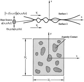
Figure 1 is a schematic representation of a rough surface contact. The highest peaks of the asperities within the nominal contact area support the load. Since the heat ¯ux is proportional to the contact pressure, the pressure must be known at every instance of time. In Fig. 1, ~x,y,z! are ®xed Cartesian coordinate axes whose origin is at the center of the nominal area. The two interacting bodies slide along the x-axis with velocities V1 and V2 . A single heat source qdx8d y 8dt8 emitted at (x8, y 8,0,t8) with no heat loss at the boundary divides itself between the two surfaces according to the heat partition function @12 f (x8, y 8,t8) #q(x8, y 8,0,t8) for surface 1 and f (x8, y 8,t8)q(x8, y 8,0,t8) for surface 2.
The temperature rise of the body 1 due to the moving point heat
source |
applied from |
time |
0 |
to t in |
nondimensional |
|
form |
|
is |
|||||||||||||
~Carslaw and Jaeger @16#! |
|
|
|
|
|
|
|
|
|
|
|
|
|
|
|
|||||||
|
|
Å |
|
|
|
|
|
|
|
|
|
|
|
|
|
|
|
|
|
|
|
|
Å |
Å |
|
t |
|
|
|
|
|
|
|
Å |
|
|
|
|
|
|
|
|
|
|
|
!5 E0 E EV |
|
|
|
|
|
|
|
|
|
|
|
|
|
|
|
|||||||
DT1~Åx,Åy ,Åz, t |
@12 f ~Åx8,Åy 8, t |
8!# |
|
|
|
|
|
|
|
|
|
|||||||||||
|
|
|
|
|
|
|
c |
|
|
|
|
|
|
|
|
|
|
|
|
|
|
|
|
|
|
|
|
|
|
|
Å |
|
|
|
Å |
|
|
|
|
|
|
|
|
|
|
|
|
Åq~Åx8,Åy 8,0, t 8 |
!dÅx8dÅy 8d t 8 |
|
|
|
|
|
|
|
|
|
||||||||||
|
|
3 |
|
|
|
|
|
|
|
|
|
|
|
|
|
|
|
|
|
|
|
|
|
|
|
|
|
|
Å |
Å |
8! |
3/2 |
|
|
|
|
|
|
|
|
|
|
|
|
|
|
|
|
|
|
|
|
|
|
|
|
|
|
|
|
|
|
|
|
||||
|
|
|
|
H |
|
|
~ t |
2 t |
|
|
|
|
|
|
|
|
|
|
|
|
J |
|
|
|
|
|
|
|
|
|
|
Å |
Å |
Å |
8!# |
2 |
1~Åy 2Åy |
8 |
! |
2 |
1Åz |
2 |
|||
|
|
3exp |
@~Åx2Åx8!2V1~ t |
2 t |
|
|
|
|||||||||||||||
|
|
2 |
|
|
|
|
|
|
|
|
|
|
|
|
|
|
|
|
||||
|
|
|
|
|
|
|
|
~Åt 2Åt 8! |
|
|
|
|
|
|||||||||
|
|
|
|
|
|
|
|
|
|
|
|
|
|
|
|
|||||||
|
|
|
|
|
|
|
|
|
|
|
|
|
|
|
|
|
|
|
|
|
(2) |
|
The corresponding temperature rise of the body 2 is:
Journal of Tribology |
Copyright © 2000 by ASME |
JULY 2000, Vol. 122 Õ 519 |
Downloaded 28 Oct 2007 to 129.5.32.121. Redistribution subject to ASME license or copyright, see http://www.asme.org/terms/Terms_Use.cfm
Both sides of Eq. ~6! are well de®ned by convolutions in the space domain.
|
|
|
|
|
|
|
|
|
|
|
|
|
|
|
|
|
|
|
|
|
|
|
|
|
|
|
|
|
|
|
|
|
|
|
|
|
|
|
|
|
|
|
|
|
|
|
|
|
|
|
|
|
|
Substituting the following de®nitions, |
|
|
|
|
|
|
|
|
|
|
|
|
||||||||||||||
|
|
|
|
|
|
|
|
|
|
|
|
|
|
|
|
|
|
|
|
|
|
|
|
|
|
|
|
|
|
|
|
|
|
|
|
|
|
|
|
|
|
|
|
|
|
|
|
|
|
|
|
|
|
|
|
|
1 |
|
|
|
|
|
H |
|
|
|
|
Å |
Å |
Å |
# |
2 |
1Åy |
2 |
J |
|
||||
|
|
|
|
|
|
|
|
|
|
|
|
|
|
|
|
|
|
|
|
|
|
|
|
|
|
|
|
|
|
|
|
|
|
|
|
|
|
|
|
|
|
|
|
|
|
|
|
|
|
|
|
|
|
Å |
8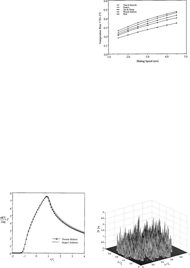
|
|
|
Å |
|
|
|
|
|
|
|
|
|
|
|
|
|
|
Å |
Å |
|
t |
Å |
|
|
|
|
Å |
|
|
|
|
|
|
|
|
!5 E0 |
|
|
|
|
|
|
|
|
|
|
|
|
|||||
T1 |
~Åx,Åy ,0,t |
$@Åq~Åx,Åy ,0,t 8!2 f q~Åx,Åy ,0,t |
8!# |
|
|
|
|
|
|
||||||||
|
|
|
|
Å |
Å |
Å |
|
|
|
|
|
|
|
|
|
(19) |
|
|
|
|
^ g1~Åx,Åy ,0,t 8!%d t 81Tb1 |
|
|
|
|
|
|
|
|
||||||
|
|
|
Å |
|
|
|
|
|
|
|
|
|
|
|
|
|
|
|
|
|
t |
|
|
Å |
|
|
|
|
|
|
Å |
|
|
|
|
|
|
5 |
E0 |
IFFT$@Åq~vÅ |
|
8!2 f q~vÅ |
|
8!# |
|
|
|
||||||
|
|
,vÅ ,0,t |
,vÅ , t |
|
|
|
|||||||||||
|
|
|
x |
y |
|
|
|
|
|
x |
|
y |
|
|
|
|
|
|
|
|
|
Å |
Å |
|
Å |
|
|
|
|
|
|
|
|
(20) |
|
|
|
|
3g1~vÅx ,vÅy ,0,t 8!%d t |
81Tb1 |
|
|
|
|
|
|
|||||||
|
|
|
Å |
|
|
|
|
|
|
|
|
|
|
|
|
|
|
Å |
Å |
|
t |
Å |
|
|
|
|
Å |
|
Å |
|
Å |
|
|
|
|
!5 E0 |
|
|
|
|
|
|
|
|
|
|
|||||||
T2 |
~Åx,Åy ,0,t |
$ f q~Åx,Åy ,0,t 8! ^ g2 |
~Åx,Åy ,0,t |
8!%d t |
8 |
1Tb2 |
|
(21) |
|||||||||
|
|
|
Å |
|
|
|
|
|
|
|
|
|
|
|
|
|
|
|
|
|
t |
|
|
Å |
|
|
|
|
|
|
Å |
Å |
|
Å |
|
|
|
5 |
E0 |
IFFT$ f q~vÅ |
|
!g |
|
~vÅ |
,vÅ |
|
8 |
|
|||||
|
|
,vÅ , t 8 |
2 |
,0,t 8!%d t |
1T |
b2 |
|||||||||||
|
|
|
x |
y |
|
|
|
x |
y |
|
|
|
|
|
|||
|
|
|
|
|
|
|
|
|
|
|
|
|
|
|
|
(22) |
|
It was stated earlier that the ¯ash temperature calculation requires a foreknowledge of the heat partition function. In transient contacts, the temperature is dependent on both the heat ¯ux dis-
Å
tribution and the Peclet (Vi) number. However, if the heat ¯ux is time-independent, Eqs. ~7!±~9! can be integrated with respect to time ®rst and then take FFT of Eq. ~11!. This allows for the heat partition function to be evaluated only once instead of at every time step.
4 Results and Discussions
The present model is based on superposition of the ¯ash temperature solutions for instantaneous moving point heat sources. Many classical solutions for the steady-state ¯ash temperature are available ~Carslaw and Jaeger @16#!. In those solutions, all the heat generated by the friction goes into one surface. Figure 2 is a comparison of the present results with those of the classical solutions for a uniform rectangular heat source whose dimensions are 2lx by 2ly along x- and y-directions respectively. The heat source is moving at a constant velocity on a semi-in®nite medium. The temperature-rise is compared along the centerline of the heat source in the direction of motion. The present solution was obtained by setting the heat partition function f (x, y ,t)50 in Eqs. ~2! and ~3! and the thermal conductivity of the surface 2 to zero. The steady-state solution is reached after a short period of time. The comparison shows a good agreement between the two solutions except for some minor differences in the region far from the heat source. These differences would be decreased when the integrating time increases and ®ner time steps are used.
Fig. 3 Comparison of maximum temperature rise for a Hertzian contact
Figure 3 shows further comparisons with existing work ~Blok @1#; Francis @6#, Tian and Kennedy @8#, Qiu and Cheng @12#!. This graph was based on a ®gure from Qui and Cheng's paper. Their contact geometry was Hertzian with one surface moving and the other stationary. The maximum contact pressure was 1.45 GPa and the nominal Hertzian contact width was 2.2631024 m. The present results most closely match with those of Qiu and Cheng. This is expected since both models are based on transient analysis. The larger differences with the other models may be attributed to approximations used for the heat partition function and the heat distribution in these steady-state models.
Figure 4 represents a typical dry contact pressure pro®le of a transversely rough sphere on a ¯at. The pressure solution was calculated based on a contact simulation technique developed by Ren and Lee @17#. It was assumed that the frictional shearing of the asperity contacts is the only source for the heat energy. Figures 5~a±c! show a transient development of the temperature pro- ®le at various stages of time during simulation. The contact surfaces were moving at velocities 2.5 m/s and 1.0 m/s in same direction. Figures 5~a!, 5~b!, and 5~c! represent the temperature distributions after 10, 50, and 200 time steps. The temperature pro®les appear surprisingly gradual although their pressure pro®le had extremely sharp peaks. This is an indication of signi®cant cross-heating activity between the asperities. Just as it is expected, an examination of the partition function showed a greater rate of heat dissipating through the faster moving surface.
Fig. 2 Comparison of the temperature solutions for a moving |
|
uniform rectangular heat source on a semi-in®nite medium. |
|
The solution is plotted at the centerline along the sliding direc- |
Fig. 4 Contact pressure distribution for a transversely rough |
tion „VslxÕ4kÄ7.56…. |
surface |
Journal of Tribology |
JULY 2000, Vol. 122 Õ 521 |
Downloaded 28 Oct 2007 to 129.5.32.121. Redistribution subject to ASME license or copyright, see http://www.asme.org/terms/Terms_Use.cfm
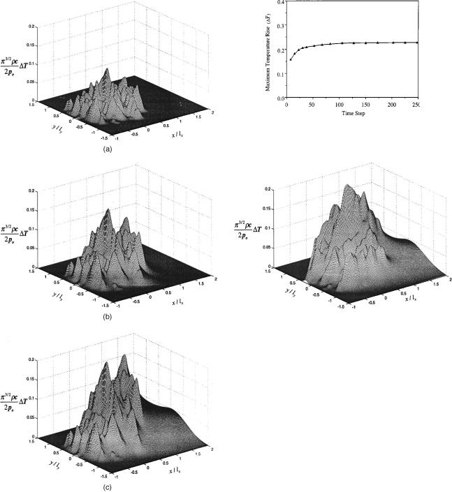
Fig. 5 „a… Flash temperature distribution for a transversely rough surface „simulation timestepsÄ10…. „b… Flash temperature distribution for a transversely rough surface „simulation timestepsÄ50…. „c… Flash temperature distribution for a transversely rough surface „steady-state solution, simulation timestepsÄ200….
The contact pressure pro®le was assumed to remain constant during simulation. The sphere and the ¯at were made of a same material and had the same bulk temperature. The coef®cient of friction, m, was set to 0.1. The simulation domain was chosen to be three times the size of the nominal contact area to reduce the periodical extension error associated with the FFT. A 4513451 grid was used for the simulation domain.
Figure 6 shows the variation of the maximum ¯ash temperature
522 Õ Vol. 122, JULY 2000
Fig. 6 Variation of maximum ¯ash temperature as a function of number of timesteps.
Fig. 7 Flash temperature distribution for a longitudinally
rough surface „steady-state solution, simulation timesteps Ä200…
as a function of time. According to the ®gure, it takes approximately 200 time steps to reach steady-state condition. The 200 time steps approximately correspond to the time it takes for the sliding velocity to cover twice the equivalent distance of the Hertzian width.
Figure 7 is a ¯ash temperature distribution for the longitudinally rough surface. The solution was found by rotating the transverse contact pressure pro®le by 90 deg. Other conditions remained the same as the previous case. The maximum nondimensional temperature rise of the longitudinal surface was higher (DTmax50.223) than that of the transverse surface (DTmax50.205). There was no obvious difference in the mean temperature since the rate of heat generation was same in both cases.
The FFT technique enables the present model to ef®ciently simulate the ¯ash temperature. This is especially useful for large number of simulation grids. As an example, if N grids are used to subdivide the simulation domain, one needs to solve N simultaneous equations for the partition function at each simulation time step. This requires O(N2) operations. Thus, as N becomes large, the computational time will signi®cantly increase. In this model, the number of ¯oating point operations is reduced to O(N log N). The total required number of ¯oating point operations for temperature, including the heat partition function calculation, is approximately 2.1 Giga-¯ops per time step. This takes about 17 seconds on a 300 MHz Power Macintosh G3.
5 Conclusions
A transient temperature model has been developed for the three-dimensionally rough surfaces in sliding contact. The simu-
Transactions of the ASME
Downloaded 28 Oct 2007 to 129.5.32.121. Redistribution subject to ASME license or copyright, see http://www.asme.org/terms/Terms_Use.cfm
lation results agree well with existing work. The present model signi®cantly reduces the computational time for the ¯ash temperature calculation. This is especially useful when simulating systems requiring a large number of grids. The FFT -based ¯ash temperature model is a powerful analytical tool enabling researchers to perform realistic asperity temperature calculations on a personal computer. The gain in ef®ciency is a result of employing FFT method in conjunction with the analytical expressions derived for the heat partition function.
Acknowledgment
The authors would like to express appreciation to Dr. Terry Mohr and The Timken Company for making this research possible.
Nomenclature
c |
5 speci®c heat of solid |
||
lx |
5 half contact length along the moving direction |
||
ly |
5 half contact length along y-direction |
||
K |
5 thermal conductivity |
||
pa |
5 asperity contact pressure |
||
Åp |
5 pa / p0 |
||
po |
5 maximum Hertzian pressure |
||
q |
5 heat ¯ux |
||
Åq |
|
|
Å |
|
5 mÅpaVs |
||
t |
5 time |
||
Å |
|
|
2 |
t |
5 4k/lx t |
||
T1b ,T2b5 bulk temperatures of bodies 1 and 2 |
|||
Å |
5 p |
3/2 |
rc/2p0T |
T |
|
||
V1 ,V2 |
5 velocities of surface 1 and 2 |
||
Vs |
5 sliding velocity uV12V2u |
||
Å |
5 Vilx/4k, i51, 2, or s |
||
Vi |
|||
x,y,z |
5 Cartesian coordinates |
||
Åx |
5 x/lx |
|
|
Åy |
5 y /lx |
|
|
Åz |
5 z/lx |
|
|
k |
5 K/rc thermal diffusivity |
||
Journal of Tribology
m |
5 friction coef®cient |
r |
5 density |
n1 ,n2 |
5 poisson's ratios of bodies 1 and 2 |
Vc |
5 real area of contact |
References
@1# Blok, H., 1937, ``Seizure Delay Method for Determining the Protection Against Scuf®ng Afforded by Extreme Pressure Lubricants,'' J. Soc. Auto Eng., 44, No. 5, pp. 175±185.
@2# Lee, S. C., and Cheng, H. S., 1991, ``Scuf®ng Theory Modeling and Experimental Correlations,'' ASME J. Tribol., 113, pp. 327±334.
@3# Blok, H, 1937, ``Theoretical Study of Temperature Rise at Surfaces of Actual Contact under Oiliness Lubricating Conditions,'' Pro. General Discussion on Lubrication, Inst. Mech. Engrs., London, 2, pp. 222±235.
@4# Jaeger, J. C., 1942, ``Moving Sources of Heat and the Temperature at Sliding Contacts,'' J. Proc. Soc., N.S.W., 76, pp. 203±224.
@5# Archard, J. F., 1959, ``The Temperature of Rubbing Surfaces,'' Wear, 2, pp. 438±455.
@6# Francis, H. A., 1971, ``Interfacial Temperature Distribution within a Sliding Hertzian Contact,'' ASLE Trans., 14, pp. 41±54.
@7# Kuhlmann-Wisdorf, D., 1987, ``Temperatures at Interfacial Contact Spots: Dependence on Velocity and on Role Reversal of Two Materials in Sliding Contact,'' ASME J. Tribol., 109, pp. 321±329.
@8# Tian, X., and Kennedy, F. E., 1994, ``Maximum and Average Flash Temperatures in Sliding Contacts,'' ASME J. Tribol., 116, pp. 167±173.
@9# Boes, J., and Moes, H., 1995, ``Frictional Heating of Tribological Contacts,'' ASME J. Tribol., 117, pp. 171±177.
@10# Ling, F. F., and Pu, S. L., 1964, ``Probable Interface Temperatures of Solids in Sliding Contact,'' Wear, 7, pp. 23±34.
@11# Lai, W. T., and Cheng, H. S., 1985, ``Temperature Analysis in Lubricated Simple Sliding Rough Contacts,'' ASLE Trans., 28, pp. 303±312.
@12# Qiu, L., and Cheng, H. S., 1998, ``Temperature Rise Simulation of ThreeDimensional Rough Surfaces in Mixed Lubricated Contact,'' ASME J. Tribol., 120, pp. 310±318.
@13# Ju, Y., and Farris, T. N., 1996, ``Spectral Analysis of Two-Dimensional Contact Problems,'' ASME J. Tribol., 118, pp. 320±328.
@14# Stanley, H. M., and Kato, T., 1997, ``An FFT-Based Method for Rough Surface Contact,'' ASME J. Tribol., 119, pp. 481±485.
@15# Ju, Y., and Farris, T. N., 1997, ``FFT Thermoelastic Solutions for Moving Heat Sources,'' ASME J. Tribol., 119, pp. 156±162.
@16# Carslaw, H. S., and Jaeger, 1959, J. C., Conduction of Heat in Solids, Oxford Press, Second Edition.
@17# Ren, N., and Lee, S. C., 1993, ``Contact Simulation of Three-Dimensional Rough Surfaces Using Moving Grid Method,'' ASME J. Tribol., 115, pp. 597±601.
JULY 2000, Vol. 122 Õ 523
Downloaded 28 Oct 2007 to 129.5.32.121. Redistribution subject to ASME license or copyright, see http://www.asme.org/terms/Terms_Use.cfm