2900

Y Delta

This function finds the N'th instance of the specified X expression range, places cursors at the two data points, and returns the difference between the Y expression values at these two points.

X Range

This function finds the X range (max - min) for the N'th instance of the specified Y range. First it searches for the specified Y Low and Y High expression values. It then searches all data points between these two for the highest and lowest X values, places cursors at these two data points, and returns the difference between the X expression values at these two points. It differs from the X Delta function in that it returns the difference in the maximum and minimum X values in the specified Y range, rather than the difference in the X values at the specified Y endpoints.

Y Range

This function is identical to the X Range function but it returns the difference in the maximum and minimum Y values in the specified X range This function is useful for measuring filter ripple.

Slope

This function finds the numeric slope at the N'th instance of the specified value of the X expression.

Options

The Monte Carlo options dialog box provides these choices:

•Status: Monte Carlo analysis is enabled by selecting the On button. To disable it, click the Off button.

•Number of Runs: The number of runs determines the confidence in the statistics produced. More runs produce a higher confidence that the mean and standard deviation accurately reflect the true distribution. Generally, from 30 to 300 runs are needed for a high confidence. The maximum is 30000 runs.

68

• Report When: This field specifies when to report a failure. The routine generates a failure report in the numeric output file when the Boolean expression in this field is true. The field typically contains a performance function specification. For example, this expression

rise_time(V(l),l,l,2,0.8,1.4)>10ns

would generate a report when the specified rise time of V(l) exceeded 10ns. The report lists the model statement values that produced the failure. These reports, included in the numeric output file (CIRCUITNAME.TNO for transient, CIRCUITNAME.ANO for AC, and CIRCUITNAME.DNO for DC), can be viewed directly and are also used by the Load MC File item in the File menu to recreate the circuits that created the performance failure.

• Distribution to Use: This choice controls the type of distribution used to generate the individual populations of component parameters.

• Gaussian distributions are governed by the standard equation

f(x) = e-.5•s•s/ • ).5

Where s = x-ji/a and ц is the nominal parameter value, a is the standard deviation, and x is the independent variable.

•Uniform distributions have equal probability within the tolerance limits. Each value from minimum to maximum is equally likely.

•Worst case distributions have a 50% probability of producing the minimum and a 50% probability of producing the maximum.

An example

To illustrate the Monte Carlo features, load the file CARLO4.CIR. This file contains a simple pulse source driving an RLC network. The circuit looks like this:

69

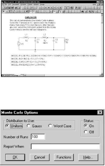
Figure 10-1 The CARLO4 circuit

Select transient analysis and then using the mouse, click the Options item from the Monte Carlo menu. It should look like this:

Figure 10-2 Monte Carlo options

The Monte Carlo options are set to run 100 runs using a Gaussian distribution. Click on the OK button and press F2 to start the runs.

70

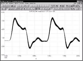
The waveforms accumulate on the screen and the result looks like this:

Figure 10-3 The analysis run

Select Monte Carlo - Histograms - Rise_Time(V(3),l,l,l,2). This selects the existing Rise_Time histogram which looks like Fig. 10-4.

This figure shows the frequency distribution for the Rise_Time performance function. The function is specified for the waveform V(3), with a Boolean of 1, which selects all data points, an N value of 1 which searches for the first rise time in the V(3) waveform, a Low value of 1.0, which defines the first level from which the rise time is to be measured, and a High value of 2.0, which specifies the second level from which the rise time is to be measured. The Rise_Time function measured one value from each of the 100 waveforms and the results are shown here in histogram form. The statistical summary a the lower left shows the lowest value, highest value, standard deviation, and mean, or average value, of the 100 numbers. The list to the right lets you scroll through individual rise time values. The Intervals

71

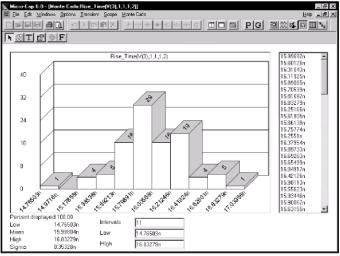
Figure 10-4 The Rise_Time histogram

value determines the number of vertical bars in the histogram. You can change the lower and upper limits in the histogram to show the percentage of the total distribution included within the limits, predicting how these limits would affect production yields.

Now we'll add a new histogram to measure the width of the pulse. Select Monte Carlo - Histograms - Add Histogram. This presents the Properties dialog box, which you use to select a performance function. Click on the Functions list box and press W to select the Width function. Click on the OK button and a new histogram is presented (Fig. 10-5).

The Width function is specified for the waveform V(3), with a Boolean of 1, which selects all data points, an N value of 1 which searches for the first pulse in the V(3) waveform, a Level of 2.0, which defines the level at which the width of the pulse is to be measured.

Press F3 to exit. Select AC from the Analysis menu. Press F2 and the screen should look like Fig. 10-6.

72

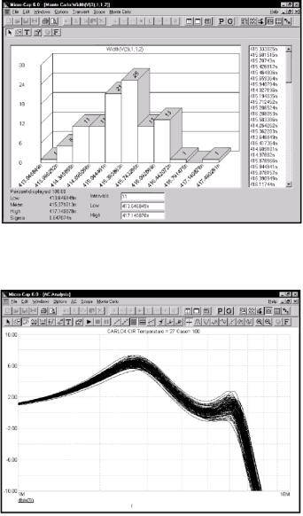
Figure 10-5 The Width histogram

Figure 10-6 100 plots of DB(V(3))

73

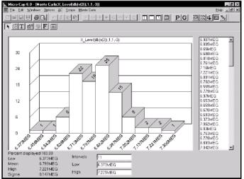
Select Add Histogram from the Histograms item on the Monte Carlo menu. From the Properties dialog box, click on the Function list box and select the X_Level function. Click in the Y Level field and type -3. Click on the OK button and a new histogram is presented. It looks like this:

Figure 10-7 AC bandwidth histogram using the X_Level function

The function is specified for the curve DB(V(3)), with a Boolean of 1, which selects all data points, an N value of 1 which finds the first X value instance in the curve, a Y Level of -3.0, which defines the level at which the X rvalue of the curve is to be measured. Since the curve is a plot of the gain of the circuit, which is a simple low pass filter, and since we chose -3 for the level, the performance function measures the 3dB bandwidth of the filter.

Press F10 to show the Properties dialog box. It includes:

Plot: This dialog box lets you change the performance function and its parameters. It lets you select one of the temperatures, had there been more than one temperature run. You can change the numeric format of the numbers used in the histogram and edit the

74

title of the histogram. If the Auto box is checked, the title automatically changes to reflect the choice and parameters of the performance function.

Color: This lets you edit the color of the histogram window parts. Font: This edits the text fonts used within the histogram plot. Tool Bar: This lets you control the histogram window tool bars. The four buttons function in the usual manner: OK: This accepts any edits and exits the dialog box. Cancel: This cancels any edits and exits the dialog box.

Apply: This updates the histogram to show the effect of the changes, which are temporary until the OK button is hit.

Help: This accesses the Help System.

Hide Window: This hides the histogram from view.

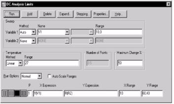
Press F3. Select DC from the Analysis menu. The Analysis Limits look like this:

Figure 10-8 The DC analysis limits

These limits specify that we plot R(R2) while stepping VI. VI has no effect on R(R2). As a result, the plots are a series of straight lines. Press F2 to start the run.

75

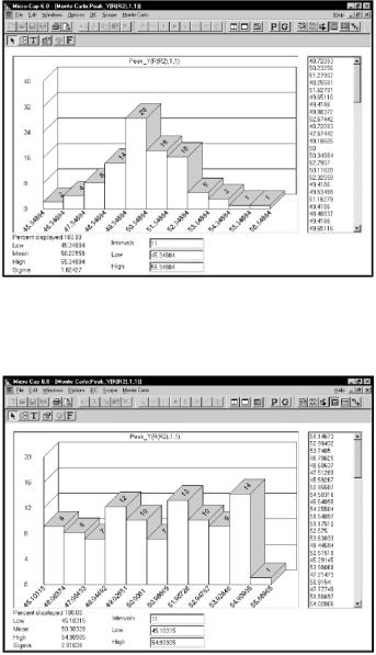
Figure 10-9 A Gaussian distribution

The Uniform distribution option produces ahistogram like this:

Figure 10-10 A uniform distribution

76

Select the Peak_Y item from Monte Carlo - Histograms. The Peak_Y function measures the largest value of R(R2), which is simply the toleranced resistor value. The distribution approximates a Gaussian distribution.

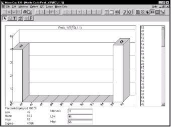
The Worst Case distribution option produces a histogram like this:

Figure 10-11A worst case distribution

In each of the three cases, we plotted the resistance value directly, so each output histogram directly mirrored the distribution function used to determine its value.

The Gaussian distribution for the resistor tolerance resulted in a similar, Gaussian output distribution. For a large number of cases, the histogram closely approaches the bell shape of the standard Gaussian equation.

The uniform distribution for the resistor produced a similar uniform output distribution, although with a few bumps. If we had run a very large number of cases, we would expect a perfectly flat histogram, reflecting an equal probability of all outputs in the range.

The worst case distribution generated an output distribution that contained the two extremes. The proportion that fall into the low or high

77