

2900
.pdfFigure 7-8 Using the Valley mode
Click on the High  button. The left cursor moves to the global high on the selected waveform.
Figure 7-9 Using the High mode
18

Click on the  button to select the Low mode. The left cursor is positioned at the right hand edge of the plot, the global low for the waveform.
Figure 7-10 Using the Low mode
Click on the Inflection  button. The left cursor moves to the next inflection point on the selected waveform. Press SHIFT + RIGHT ARROW key. The right cursor moves to the next inflection point on the selected waveform moving right (Fig, 7-11).
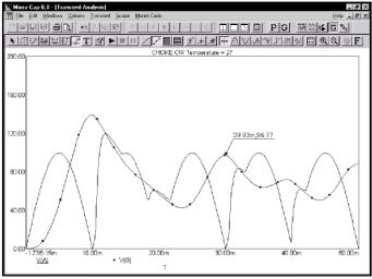
Click on the Go to Y  button. Type "50" in the dialog box that comes up and click on the 'Left' button in the dialog box. The left cursor is positioned at the first incidence of 50.0 for the selected waveform's Y expression value (Fig, 7-12).
19
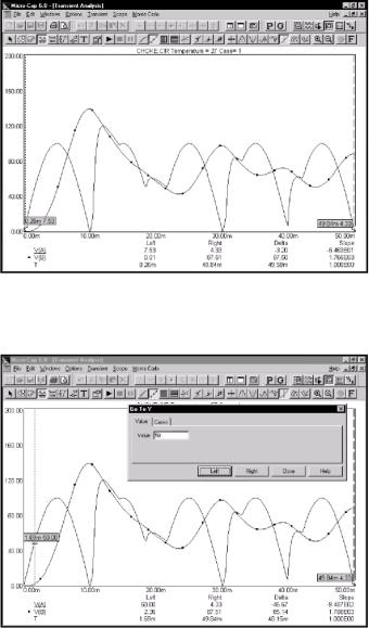
Figure 7-11 Using the Inflection mode
Figure 7-12 Using the Go to Y mode
20
Задание 2
Прочтите и ответьте на вопросы.
1.Каким образом добавляется текст на выбранные участки?
2.Как выполняется измерение характеристик?
3.Найдите и поясните рисунки, демонстрирующие измерение времени нарастания и спада импульсов.
4.В чем заключаются возможности анимации анализа?
Adding text to plots
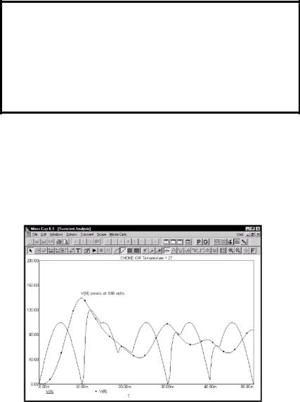
Adding text to an analysis plot is easy. Click on the Close button to
exit the Go To Y mode. Click on the  button to select the Text mode. Click the mouse near the large peak of the V(B) waveform and type "V(B) peaks at 138 volts.". Click OK. The screen looks like this:
Figure 7-13 Adding text to a plot
21
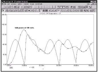
Would the text look better if it were centered over the peak? To see if it would, first enter Select mode by pressing the SPACEBAR or by
clicking on the Select button  . Next, click on the text with the left button and drag it to the left until it is centered. Release the button and the text is redrawn at the mouse position.
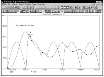
Perhaps the text would look better if it were bold. Double click on the text and when the text dialog box is presented, click on the Font tab in the dialog box. This part of the dialog box lets you change the font and several font attributes. In this case, we need to change the Style attribute. From the Font Style group, select the Bold option. Click on the OK button. The text should now appear as in Figure 7-14. All font attributes for each instance of text are independently changeable.
Figure 7-14 Changing the font style of the text
Adding tags to plots
Click on the  button to activate the Vertical Tag mode. Click the left mouse button near the highest peak of V(A). Drag the mouse to the highest peak of V(B) and release the button. The tag shows the vertical delta between the two data points. (Fig, 7-15).
22
In a similar manner, the horizontal tag, enabled by the  button, measures the horizontal delta between the two data points of the tag. It is most useful for measuring the time difference between two digital events, such as the width of a pulse or the time delay between two events. Choose Delete All Objects from the Scope menu to delete the text and tag.
Figure 7-15 Using the Vertical tag mode
'Click on the  button to activate the Point Tag mode. Click the left mouse button at the second peak of V(B) and drag the mouse. The point tag labels the actual analysis data point nearest the initial mouse click. A shadow of the tag will track the mouse movements. Release the mouse button when the shadow is at the desired spot. The screen should look like Figure 7-16.
When in Select mode, double clicking on a tag element invokes the Tag dialog box. This dialog box lets you edit the arrow style, weight, color, and the font attributes of the number. All of the tag options are available for each instance of a tag element.
23
Both the text body and arrow tip of a tag may be repositioned after placement. To reposition, first enable the Select mode. Click on the tag and then drag either the body handle or the arrow tip handle. The body handle is the small black rectangle near the text. The arrow tip handle is the small black rectangle at the tip of the tag arrow.
Press F3 to exit the analysis, then CTRL + F4 to close the file.
Figure 7-16 Using the Point tag
Performance functions
MC6 provides a group of functions for measuring perfor- mance-related curve characteristics. These functions include:
Rise Time
This function marks the N'th time the Y expression rises through the specified Low and High values. It places the cursors at the two data points and returns the difference between the X expression values at these two points. This function is useful for measuring the rise time of time-domain waveforms.
24
Fall Time
This function marks the N'th time the Y expression falls through the specified Low and High values. It places the cursors at the two data points and returns the difference between the X expression values at these two points. This function is useful for measuring the fall time of time-domain waveforms.
Peak X
This function marks the N'th local peak of the selected Y expression. A peak is any data point algebraically larger than the neighboring data points on either side. It places the left or right cursor at the data point and returns its X expression value.
Peak Y
This function is identical to the Peak X function but returns the Y expression value. This function is useful for measuring overshoot in time-domain waveforms and the peak gain ripple of filters in AC analysis.
Valley X
This function marks the N'th local valley of the selected Y expression. A valley is any data point algebraically smaller than the neighboring data points on either side. It places the left or right cursor at the data point and returns its X expression value.
Valley Y
This function is identical to the Valley X function but returns the Y expression value. It is useful for measuring undershoot in time-domain waveforms and the peak attenuation of filters in AC analysis.
PeakJValley
This function marks the N'th peak and N'th valley of the selected Y expression. It places the cursors at the two data points and returns the difference between the Y expression values at these two points. This function is useful for measuring ripple, overshoot, and amplitude
Period
The period function accurately measures the time period of waveforms by measuring the X differences between successive
25
instances of the average Y value. It does this by first finding the average of the Y expression over the simulation interval where the Boolean expression is true. Then it searches for the N'th and N+l'th rising instance of the average value. The difference in the X expression values produces the period value. Typically a Boolean expression like "T>500ns" is used to exclude the errors introduced by the non-periodic initial transients. This function is useful for measuring the period of oscillators and voltage to frequency converters, where a waveform's period usually needs to be measured to high precision.
Frequency
This is the numerical complement of the Period function. It behaves like the Period function, but returns 1/Period. The function places cursors at the two data points.
Width
This function measures the width of the Y expression curve by finding the N'th and N+l'th instances of the specified Level value. It then places cursors at the two data points, and returns the difference between the X expression values at these two points.
High X
This function finds the global maximum of the selected branch of the selected Y expression, places either the left or the right cursor at the data point, and returns its X expression value.
High Y
This function acts like High X, but returns the Y value.
Low X
This function finds the global minimum of the selected branch of the selected Y expression, places either the left or the right cursor at the data point, and returns its X expression value.
Low Y
This function acts like Low_X, but returns the Y value.
26
X Level
This function finds the N'th instance of the specified Y Level value, places a left or right cursor there, and returns the X expression value.
Y Level
This function finds the N'th instance of the specified X Level value, places a left or right cursor there, and returns the Y expression value.
X Delta
This function finds the N'th instance of the specified Y expression range, places cursors at the two data points, and returns the difference between the X expression values at these two points.
Y Delta
This function finds the N'th instance of the specified X expression range, places cursors at the two data points, and returns the difference between the Y expression values at these two points.
X Range
This function finds the X range (max - min) for the N'th instance of the specified Y range. First it searches for the specified Y Low and Y High expression values. It then searches all data points between these two for the highest and lowest X values, places cursors at these two data points, and returns the difference between the X expression values at these two points. It differs from the X Delta function in that it returns the difference in the maximum and minimum X values in the specified Y range, rather than the difference in the X values at the specified Y endpoints.
Y Range
This function is identical to the X_Range function but it returns the difference in the maximum and minimum Y values in the specified X range This function is useful for measuring filter ripple.
27