2900

• Vertical Axis Grids: This adds grids to the vertical axis.

• Minor Log Grids: This adds minor log grid lines between the major grids to any axis which uses the log option.

• Baseline: This adds a plot of the value 0.0 for use as a reference.

• Horizontal Cursor: This adds a horizontal cursor intersecting each of the two vertical numeric cursors at their respective data point locations.

•Trackers: These options control the display of the cursor, intercept, and mouse trackers, which are little boxes containing the numeric values at the current data point, its X and Y intercepts, or at the current mouse position.

•Cursor Functions: These control the cursor positioning in Cursor mode. Cursor positioning is described later in this chapter.

• Animate Options: This option displays the node voltages/states, and optionally, device currents, power, and operating conditions (ON, OFF, etc.), on the schematic as they change from

one data point to the next. To use this option, click on the button, select one of the wait modes, then click on the Tile Hori-

zontal button, or Tile Vertical button, then start the run. If the schematic is visible, MC6 prints the node voltages on analog nodes and the node states on digital nodes. To print device cur-

rents click on . То print device power click on . To print the

device conditions click on . It lets you see the evolution of states as the analysis proceeds. To restore a full screen plot, click

on the button.

• Normalize at Cursor: (CTRL + N) This option normalizes the selected (underlined) curve at the current active cursor position. The active cursor is the last cursor moved, or if neither has been

8

moved, then the left cursor. Normalization divides each of the branch's Y values by the Y value of the branch at the current cursor position, producing a normalized value of 1.0 there. If the Y expression contains the dB operator and the X expression is F (Frequency), then the normalization subtracts the value of the Y expression at the current data point from each of the curve's data points, producing a value of 0.0 at the current cursor position.

• Go to X: (SHIFT + CTRL + X) This command lets you move the left or right cursor to the next instance of a specific value of the X expression of the selected waveform. It then reports the Y expression value at that data point.

• Go to Y: (SHIFT + CTRL + Y) This command lets you move the left or right cursor to the next instance of a specific value of the Y expression of the selected waveform. It then reports the X expression value at that data point.

• Go to Performance: This command calculates performance function values on the Y expression of the selected curve. It also moves the cursors to the measurement points. For example, you can measure pulse widths and band widths, rise and fall times, delays, periods, and maxima and minima.

•Tag Left Cursor: (CTRL + L) This command attaches a tag to the left cursor data point on the selected curve.

•Tag Right Cursor: (CTRL + R) This command attaches a tag to the right cursor data point on the selected curve.

•Tag Horizontal: (SHIFT + CTRL + H) This command drags a horizontal tag from the left to the right cursor, showing the difference between the two X expression values.

•Tag Vertical: (SHIFT + CTRL + V) This command drags a vertical tag from the data point at the intersection of the curve and the left cursor to the intersection of the curve and the right cursor, showing the difference between the two Y expression values.

9

•Align Cursors: This option, available only in Cursor mode, forces the left and right cursors of different plot groups to stay on the same data point.

•Keep Cursors on Same Branch: When stepping produces multiple runs, one line is produced for each run for each plotted expression. These lines are called branches of the curve or expression. This option forces the left and right cursors to stay on the same branch of the selected curve when the UP ARROW and DOWN ARROW cursor keys are used to move the numeric cursors among the several branches. If this option is disabled the cursor keys will move only the left or right numeric cursors, not both, allowing them to occupy positions on different branches of the curve.

•Same Y Scales: This option forces all curves in a plot group to use the same Y scale. Otherwise, if the curves have differing Y Range values, one or more Y scales will be drawn.

Next, choose Mode from the Options menu. The five modes beginning with Scale deal with analysis plots and are usually accessed by clicking on their Tool bar buttons shown below, but they may also be activated from this menu.

• Scale: In this mode, the left mouse button drags an outline box to magnify a portion of the plot. F7 also accesses this mode.

• Cursor: This mode shows the numeric value of each waveform at each of two plot cursors. The left mouse button controls the left plot cursor and the right button controls the right plot cursor. The left cursor is initially placed on the first data point. The right cursor is initially placed on the last data point. The LEFT ARROW or RIGHT ARROW keys move the left or right cursor to a point on the selected waveform. Depending on the positioning mode, the point may be the next local peak or valley, global high or low, inflection point, or simply the next data point. The direction is left or right depend-

10

ing on whether a LEFT ARROW or RIGHT ARROW key is pressed. If the SHIFT key is used with the cursor key, the right cursor is moved, otherwise, the left cursor is moved. F8 may also be used to access this mode.

• Point Tag: In this mode, the left mouse button is used to tag a data point with its numeric (X,Y) value. The tag snaps to the nearest data point.

• Horizontal Tag: In this mode, the left mouse button can be used to drag between two data points to measure the horizontal difference.

• Vertical Tag: In this mode, the left mouse button can be used to drag between two data points to measure the vertical difference.

Note:

In all modes except Cursor mode, a drag of the right mouse button pans the schematic. In Cursor mode, CTRL + right mouse drag pans the schematic.

Magnifying

Press ESC twice to remove the menus. Click the left mouse button just above and to the left of the large peak of the V(B) waveform. While holding the left button down, drag the mouse down and to the right to create a magnification box like the one shown in Figure 7-3.

11

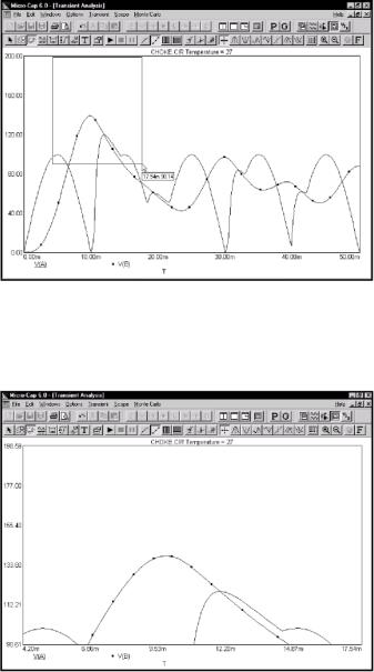
Figure 7-3 Magnifying a region

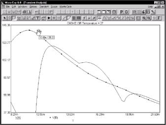
Release the button and MC6 scales the plot to match the outline of the box.

Figure 7-4 The magnified region

12

Panning

Panning is like scrolling in a text field, except that it is multidirectional. To illustrate, click the right mouse button in the middle of the plot. The mouse arrow cursor changes to a hand cursor. While holding the right button down, drag the mouse slowly up and to the left until it nearly touches the upper left corner of the plot window. The effect is like sliding a paper across a desk. Dragging the mouse dynamically updates the display to reflect the change in view. Release the button and the plot looks like this:

Figure 7-5 Panning the plot

As with panning in the Schematic editor, the keyboard may also be used. The CTRL key plus the arrow keys move the view in the direction of the arrow.

The combination of panning and magnifying allows close inspection of any portion of the waveforms.

Note that you can also scale (magnify) and pan while in Cursor mode:

13

Scaling: CTRL + left mouse drag

Panning: CTRL + right mouse drag for panning.

Press CTRL + HOME or choose Restore Limit Scales from the Scope menu to return the analysis to its original offset and scale.

Cursor mode

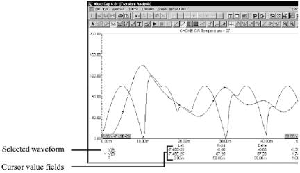
Click on the Cursor mode button or Press F8 to place Scope in the Cursor mode. In this mode the display looks like this:

Figure 7-6 The Cursor mode

The Cursor value fields, located below the plots, show the numeric value of each waveform or expression at both cursor positions. The X expression value is shown below the Y expression values. The purpose of each field is as follows:

•Left: This shows the value of the row's Y expression at the left cursor.

•Right: This shows the value of the row's Y expression at the right cursor.

14

•Delta: This shows the value of the row's Y expression at the right cursor minus the value of the Y expression at the left cursor.

•Slope: This shows the row's Y expression delta value divided by the delta value of the X expression. If the X expression is Т (time), then this field approximates the time derivative of the waveform between the two cursors. The slope calculation can be changed to dB/Octave or dB/Decade from

•Properties / Scales and Formats, if dB is used in the Y expression and F (frequency) is the X expression.

Cursor mode panning and scaling

Mouse

Normal mouse-controlled scaling and panning are not available in Cursor mode, since the mouse movements in this mode are used to control the left and right waveform cursors. However, by using the CTRL key together with the mouse, you can pan and scale within Cursor mode as follows:

To scale (magnify) the waveforms, press the CTRL key down and drag with the left mouse button.

To pan the waveforms, press the CTRL key down and drag with the right mouse button.

Keyboard

To pan the waveforms with the keyboard, press the CTRL key down and press the LEFT ARROW or RIGHT ARROW keys.

There is no keyboard-based scaling procedure.

15

Cursor mode positioning

Drag with the left mouse button to control the left cursor, and the right button to control the right cursor. The LEFT ARROW and RIGHT ARROW cursor keys move the left cursor and SHIFT + cursor keys move the right cursor. The mouse places the cursor anywhere, even between simulation data points. The keyboard moves the cursor to one of the simulation data points, depending on the positioning mode. The positioning mode, chosen with a Tool bar button, affects where the cursor is placed the next time a cursor key is pressed. Cursor positioning picks locations on the selected, or underlined, curve. Waveforms are selected with the Tab key, or by clicking the Y expression with the mouse.

• Next: This mode finds the next data point on the selected curve.

• Peak: This mode finds the next local peak on the selected curve.

• Valley: This mode finds the next local valley on the selected curve.

• High: This mode finds the data point with the largest algebraic value on the current branch of the selected curve.

• Low: This mode finds the data point with the smallest algebraic value on the current branch of the selected curve.

• Inflection: This mode finds the data point with the largest magnitude of slope, or first derivative, on the selected curve.

• Global High: This mode finds the data point with the largest algebraic value on all branches of the selected curve.

• Global Low: This mode finds the data point with the smallest algebraic value on all branches of the selected curve.

16

When Cursor mode is selected, a few initialization events occur. The selected curve is set to the first, or top waveform. The Next mode is enabled. Clicking on a mode button not only changes the mode, it also moves the last cursor in the last direction. The last cursor is set to the left cursor and the last direction is set to the right. The left cursor is placed at the left on the first data point. The right cursor is placed at the right on the last data point.

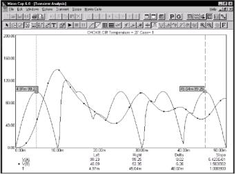
Click on the Peak button. The left cursor moves to the first peak to the right of its current position on the selected waveform, V(A). Press SHIFT + LEFT ARROW key. The right cursor moves to the first peak on its left.

Figure 7-7 Using the Peak mode

Click on the button to select the Valley mode. Press the RIGHT ARROW key. The cursors are placed on the next valley in the right and left directions.

17