Geomagnetic_Disturbance_Task_Force_2012

Chapter 4–GMD Credible Threat Definition

to magnetic east (D) and vertically down (Z). The conversion from H, D, Z to X, Y, and Z depends on the magnetic declination at each observatory. In North America, the magnetic observatories are operated by the United States Geological Survey (USGS) and the Geological Survey of Canada (GSC). Magnetic data are available from these institutes and also through the InterMagnet website.51

The digital geomagnetic data can be used to determine the rate of change of the magnetic field dB/dt. The occurrence of peak values of the rate of magnetic field change in time (dB/dt) in each hour evaluated. Figure 9 shows the percentage occurrence of dB/dt greater than 300 nT/minute derived from Canadian and U.S. magnetic observatories. The results vary smoothly with the geomagnetic latitude of the observatory, so the results were extrapolated along lines of constant geomagnetic latitude to produce the contour lines of occurrence. These relative percent expectations show an extremely low probability for large events in most of North America.

Figure 9: Percent probability of occurrence of hourly peak dB/dt greater than 300 nT/min.

4.3.3 Geomagnetic Substorms

A geomagnetic substorm, sometimes referred to as a magnetospheric substorm, is a brief disturbance in Earth's magnetosphere that causes energy to be released from the “tail’ of the magnetosphere and injected into the high latitude ionosphere. Substorms usually take place over a period of a few hours and are observable primarily at the Polar Regions. Substorm

51 Intermagnet is available at: http://www.intermagnet.org

Chapter 4–GMD Credible Threat Definition

occurrence becomes more frequent during a geomagnetic storm when one substorm may start before a previous one has completed. The recent launch of the multi satellite NASA THEMIS mission was specifically designed to look at issues surrounding substorms. This work is on going.

4.3.4 Calculation of Electric Fields

The magnetic field variations that occur during a GMD induce electric fields on Earth. These electric fields drive current flows (GIC) on Earth that tends to cancel the magnetic field variations, producing a fall off in amplitude with depth. This is the well known “skin effect” seen in conductors. However, because of Earth’s lower conductivity, the skin depth is much greater than in metals, and the fields penetrate to depths ranging from kilometers to hundreds of kilometers depending on the frequency. At the frequencies of concern for GIC (seconds to hours), the magnetic field variations penetrate the thin surface layer of soil; the conductivity of this layer has no influence. Earth conductivity at depths into the crust and mantle influences the electric fields on the surface of Earth; this needs to be taken into account when calculating the electric fields and resulting GIC.

Information about the conductivity structure of Earth can be obtained from magnetotelluric soundings, with interpretation aided by consideration of other geophysical and geological information. The basic tectonic structure of North America consists of ancient rocks of the Canadian Shield, sedimentary rocks to the south and west, and the uplifted rocks that form the Appalachian Mountains on the east coast and the Cordilleran Mountains on the west coast. In the southeast United States, there are also coastal plains between the mountains and the oceans. This information can be used to produce a layered model that represents Earth’s conductivity structure below the region of a specific power system (see Figure 10). The Québec model shows the high resistivity in the upper 15 km characteristic of the Canadian Shield, whereas the British Columbia model shows more conductive upper layers. These models represent the upper and lower range of resistivity. Models for other regions would be expected to have values at or between these two extremes.

The one dimensional Earth models (i.e., only considering variation with depth) can be used to calculate the surface impedance of Earth. This is effectively the transfer function of Earth, showing the frequency domain relation between the electric and magnetic fields on Earth’s surface. Thus, the electric fields can be calculated by creating a Fourier transform of the time series of magnetic field data, multiplying the magnetic field spectrum by Earth’s surface impedance to obtain the electric field spectrum, and then inversing the resulting Fourier transform to convert this to the time series of electric field values.

Electric field values have been calculated for a number of observatories in North America. Figure 11 shows the hourly peak electric field values as a function of the activity index Kp. This can be combined with the statistics of Kp shown in Figure 8 above to estimate the occurrence of electric field values.

Chapter 4–GMD Credible Threat Definition

Figure 10: Examples of Earth conductivity models

Figure 11: Occurrence of hourly peak electric fields for different Kp values

An alternative approach is to use the available archive of digital magnetic field data to calculate the electric fields that occurred during the data interval. A statistical analysis can then be made directly on the electric field values.

Chapter 4–GMD Credible Threat Definition

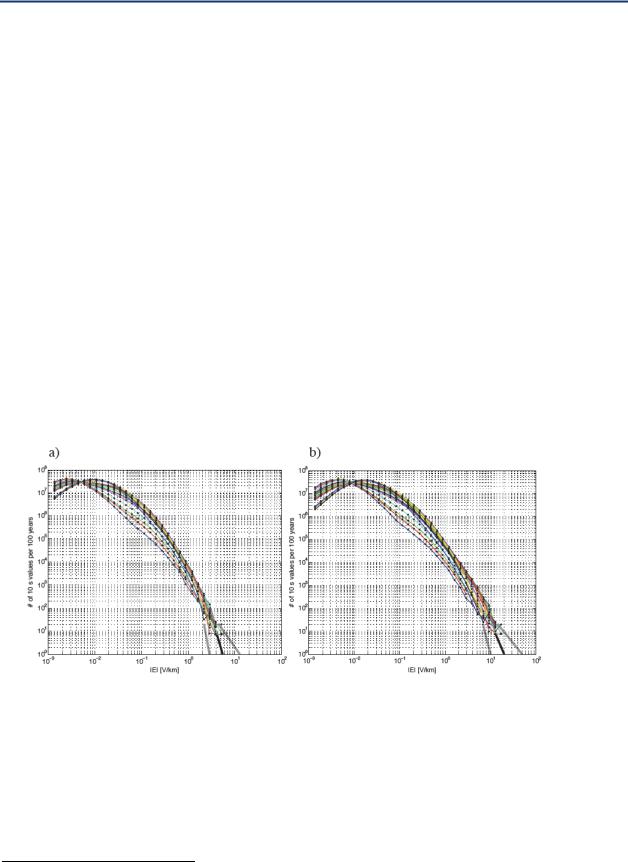
To provide an example of this information use, a recent analysis was completed by using geomagnetic data with 10 second sampling from 1993 to 2006 and the resistive and conductive Earth models in Figure 10 to calculate electric fields using geomagnetic data from the NASA Imager for Magnetopause to Aurora Global Exploration (IMAGE) chain.52 A statistical analysis of these values (see Figure 12) shows the decrease in occurrence with increasing amplitude, which is then extrapolated to determine the electric field magnitude expected once in a 100 years. For a conductive Earth structure, Figure 12a indicates a 100 year peak electric field of 5 V/km for British Columbia, while for a resistive Earth structure Figure 12b indicates a 1 in 100 year peak electric field value of 20 V/km for Québec.

The amplitude of geomagnetic disturbances (and hence the peak electric fields) also shows a strong dependence on latitude. It is valuable to calibrate the magnetic field data recorded at the North American geomagnetic observatories during the March 13 14, 1989, and October 29 31, 2003, geomagnetic disturbances with the aforementioned calculations. Figure 13 shows the peak electric field values occurred in the auroral zone and a dramatic drop at a geomagnetic latitude threshold of about 50 degrees. More information and background can be found in

Generation of 100 year geomagnetically induced current scenarios. 53.

Figure 12: Statistical occurrence of geoelectric fields calculated using the ground conductivity structure of (a) British Columbia (conductive) and (b) Québec (resistive).

Note: Different curves correspond to different IMAGE stations used in the computation of the geoelectric field. The black lines indicate approximate visual extrapolations of the statistics to 100 year peak magnitudes. The gray lines indicate the reasonable lower and upper boundaries for the extrapolated values.

52The NASA IMAGE Chain is available at: http://image.gsfc.nasa.gov/

53Pulkkinen, A., E. Bernabeu, J. Eichner, C. Beggan and A. Thomson, Generation of 100 year geomagnetically induced current scenarios, Accepted for publication in Space Weather, 2012.

Chapter 4–GMD Credible Threat Definition

Figure 13: Spatial distributions of the maximum computed geoelectric field for (a) March 13 15, 1989 and (b) October 29 31, 2003.

Note: The center of each circle indicates the location of the corresponding magnetometer station and the radius of the circle indicates the maximum magnitudes of the physical parameters.

To provide an example of the geoelectric fields that could occur during a one in 100 year scenario (also referred to as the GIC test wavefronts) at different latitudes and with regions of different resistivity, geoelectric fields calculated for the October 29, 2003, event for the Nurmijarvi and Memanbetsu magnetic observatories were scaled to determine the peak electric fields expected from Figures 11 and 12. The results, shown in Figure 14, indicate that above the threshold geomagnetic latitude, the peak electric fields are 20 V/km and 5 V/km in resistive and conductive regions respectively. Below the threshold geomagnetic latitude, the corresponding peak electric fields are 2 V/km and 0.5 V/km for resistive and conductive regions.

Chapter 4–GMD Credible Threat Definition

Figure 14: Illustration of extreme horizontal geoelectric field scenarios (X indicates geographic north, Y indicates geographic east)

Note that the vertical scales are different in different panels.

Panel a): Scenario for resistive ground structures for locations above the threshold geomagnetic latitude. The maximum geoelectric field amplitude is 20 V/km. Panel b): Scenario for conductive ground structures for locations above the threshold geomagnetic latitude. The maximum geoelectric field amplitude is 5 V/km. Panel c): Scenario for resistive ground structures for locations below the threshold geomagnetic latitude. The maximum geoelectric field amplitude is 2 V/km. Panel d): Scenario for conductive ground structures for locations below the threshold geomagnetic latitude. The maximum geoelectric field amplitude is 0.5 V/km.

Chapter 5–Power Transformers

5.Power Transformers

5.1 Introduction

This chapter addresses the potential for shortened lifespan and/or failure of power transformers from geomagnetic disturbances. This issue is of paramount importance. Evidence from several solar storm events suggests that GIC can have an impact on some EHV transformer designs and those nearing the end of life. The primary threat to power transformers is the heating of windings, and other structural parts, as well as the corresponding winding loss of life. Heating induced by half cycle saturation as a potential failure mechanism in transformers, while the loss of reactive power supply also caused by half cycle saturation in transformers, is addressed in Chapter 8 (Modeling GIC).

In some cases, the effect of GIC in individual power transformers can be significant and warrants attention, analysis, and possible mitigation.

5.2 Basics of GIC Effects on High Voltage Power Transformers

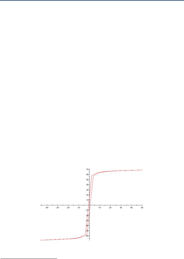
The flux current characteristic of transformer core materials is non linear (see Figure 15). During normal steady state operation, transformers are designed so the flux is in the linear region. If a transformer operates outside nominal voltage design values (typically greater than 1.1 per unit) the peak flux density can reach the saturation range of the core, forcing the magnetic flux into other parts of the transformer. In such cases, the magnetizing current is no longer sinusoidal and has relatively large current peaks, as shown in Figure 16. In addition to the positive and negative currents peaks, the current also shows some distortion due to hysteresis.54

Figure 15: Transformer magnetizing characteristic for a 100 MVA, 115/27 kV, single phase transformer

Flux (Volt-s)

Magnetizing current (A)

54The behavior of the magnetizing characteristic of a transformer is different when the flux in the core is increasing than when it is decreasing because it takes energy to reorient the magnetic field in the core. This effect is called hysteresis.

Chapter 5–Power Transformers

Figure 16: Transformer magnetizing current during saturation

When a power transformer is subjected to DC currents during steady state operation, a unidirectional, or DC flux, is impressed in the core. The magnitude of this DC flux depends on the magnitude of the DC current, the number of turns in the windings carrying the DC current, and the reluctance of the path DC. The DC flux adds to the AC flux during half the 60 Hz cycle and subtracts from the AC flux during the other half, thus shifting the operating point of the magnetizing characteristic (see Figure 17). This phenomenon is often referred to in the technical literature as half cycle saturation. With a DC offset, the magnetizing current is neither sinusoidal nor symmetrical, and has relatively large current peaks on the positive or negative side of the cycle (but not both), as shown in Figure 18.

The larger the DC flux, the larger the magnetizing current peak (see Figure 19). For instance, Figure 19 shows an Electromagnetic Transients Program (EMTP) simulation (of the 100 MVA, 115/27.6 kV transformer whose characteristic is shown in Figure 15) where the DC bias of the flux is continually increased to illustrate the increase of peak currents during half cycle saturation. For large values of peak current, the effect of hysteresis is negligible. As a point of reference, the root mean square (rms) magnetizing current for this transformer under normal operating conditions is 2.2 amps.

Chapter 5–Power Transformers

Figure 17: Relationship between flux and current with and without DC flux

Saturated

B

Unsaturated

Half-cycle saturation currents

Normal currents

Time

Figure 18: Transformer magnetizing current during half cycle saturation (0.8 amps/phase)

Chapter 5–Power Transformers

Figure 19: Transformer magnetizing current for increasing values of DC current per phase

The magnetizing current peak values (and under high levels of GIC, the rms values) can become a substantial portion of the nominal rated current of the transformer during half cycle saturation. The numerical values shown are based on ElectroMagnetic Transients Program (EMTP) simulations that illustrate the physics of the phenomenon from a power system point of view. Also, as further discussed in Section 5.3 below, the magnetizing characteristic and how DC flux offset is affected when DC currents flow (GICs) through the windings can vary depending on many factors, such as core construction and design characteristics. The duration of this pulse is only in the range of 1/6th to 1/10th of the cycle; once per cycle. Figure 20 illustrates different magnetizing current peak values as a function of GIC for a single phase unit.