Geomagnetic_Disturbance_Task_Force_2012

Attachment 8–Example of GIC Calculation

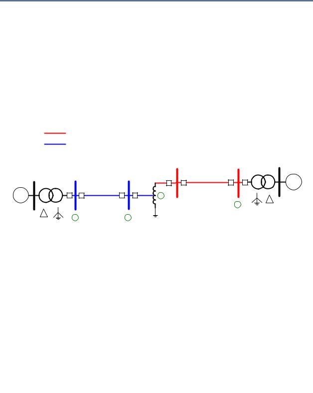
Figure A8 1: Induction process and system model

Vdc E dl

The following sections describe the models necessary to compute GIC.

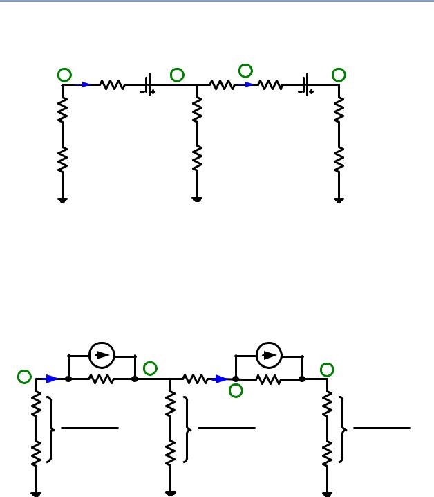
A8.2.1 Transmission Line Models

Slow varying dB/dt results in an induced voltage in the millihertz range. Thus, the induced voltage can be modeled as purely DC, and the system can be modeled by a resistance network (i.e., mutual coupling, inductance and shunt capacitance can be ignored). A three phase transmission line model that can be used for GIC calculation is shown in Figure A8 2.

Figure A8 2: Transmission line model

The quasi DC voltage that is induced in each phase of a transmission line can be computed using Faraday’s Law as defined in (1):

Attachment 8–Example of GIC Calculation

where E is the induced geoelectric field at the surface of Earth, and dl is the incremental length of the transmission line including direction. For the purposes of GIC calculations, it is assumed that the electric field at the height of the transmission line is equal to the electric field at Earth’s surface. If the geoelectric field can be assumed constant in the geographical area of a transmission line, then only the coordinates of the end point of the line are important,

regardless of routing twists and turns. The resulting incremental length vector dl , becomes L .

The vector L , representing the length and direction of the line between end points can be constructed using an arbitrary reference; however, such a method can introduce error. An improved method is to compute the distance in the x and y directions independently. Recall that the dot product of two vectors A and B can be computed using (2):

where Ex is the northward electric field (V/km), Ey is the eastward electric field (V/km), Lx is the northward distance (km), and Ly is the eastward distance (km).

The following procedure can be used to compute northward and eastward distances. Consider a transmission line between substations A and B. The northward distance can be computed using (4):

where ∆lat is the difference in latitude (degrees) between the two substations A and B. The eastward distance can be computed using (5):

Ly 111.2 long sin 90 (5)

where ∆long is the difference in longitude (degrees) between the two substations A and B, andis defined in (6) as the average of the two latitudes:

The line resistance that is modeled is simply the DC resistance of the line. If this value is unavailable, it can be derived from the positive sequence resistance of the line using a correction factor to account for skin effect. The correction factor varies from approximately 0.95 for large conductors (e.g., 1,590 MCM), to unity for smaller conductors (e.g., 750 MCM) [2]. Specific correction factors can be determined from conductor tables. When possible, the DC resistance corresponding to the line operating temperature should be used.

Attachment 8–Example of GIC Calculation

A8.2.2 Transformer Model

Calculating GIC requires a modification in the way in which transformers are modeled. In the case of GIC calculations, only the winding resistance is modeled, and induction between the windings is ignored. Figure 3 shows the three phase equivalent circuit of several common types of transformer winding configurations. Note that transformer windings without terminal designations are ignored in the analysis. This corresponds to all delta windings (as shown in Figure 3) and ungrounded wye windings (not shown).

Figure A8 3: GIC models of common transformer winding configurations

Attachment 8–Example of GIC Calculation

The resistance that is modeled is the DC winding resistance of the transformer. This information can be obtained from transformer test reports, but is not always available. The following assumptions can be used when test report data are unavailable.

The resistance of grounded wye, two winding transformers can be approximated from the positive sequence resistance that is available in power flow and short circuit databases. The assumption is made that the primary winding resistance and the referred value of the secondary winding resistance of the transformer are approximately equal [2]. In other words, one half of the per unit resistance is modeled on the high voltage winding, and one half of the per unit resistance is modeled on the low voltage winding. The per unit resistance is then converted to ohms using the appropriate base quantities.

Grounded wye autotransformers are modeled in a similar manner using the resistance measured from the H terminal to the X terminal with the X terminal short circuited (i.e., RHX). This resistance consists of a sum of the series winding resistance and the referred value of the common winding resistance, with referral based on the ratio of the series winding voltage to the common winding voltage:

where n VH .

VX

A8.2.3 Substation Ground Grid Model

Equivalent station grounding resistance to remote Earth, Rg, should be modeled. This is the equivalent resistance of the station grounding mat and the ground wires of all transmission circuits connected to the station grounding mat.

A8.2.4 Miscellaneous Modeling Details

Shunt reactors and shunt capacitors do not have to be modeled. Shunt capacitors represent an infinite resistance to near DC currents, shunt reactors are normally connected to tertiary transformer windings, and they are largely decoupled from the DC network. HV line reactors can be included in the network, but their resistance is usually larger than the transformer winding resistance, and their effect is minimal.

Transmission lines below 230 kV are typically not modeled because the resistances of conductors used in lines 115 kV and below are usually much higher than those used in circuits 230 kV and above.

Interconnections to other utilities can be modeled as a transmission line terminated in a transformer. Normally the approximate geographical orientation and length of the line to the neighboring utility transmission station is known, and generic resistance values can be used based on voltage level and interconnection capacity.

Attachment 8–Example of GIC Calculation

A8.3 Example Calculation of GIC in HV and EHV Networks

The following section describes the steps that can be taken to compute GIC flow in a power system.

The network can be modeled as a single phase network because the spatial distances between conductors of a transmission circuit are negligible compared to the distance of the transmission circuit to the electrojet. The example six bus system that will be analyzed is shown in Figure A8 4. Bus numbers are shown at bus locations. Encircled numbers refer to circuit nodes that will be used later in the calculation of GIC.

Figure A8 4: Example system used to compute GIC

Required system data are provided in Tables A8 1and A8 2.

Table A8 1: Substation location and ground grid resistance

Table A8 2: Transmission line information

Attachment 8–Example of GIC Calculation

Table A8 3: Transformer and autotransformer winding resistance values

For these calculations we use the geomagnetic coordinate system with x axis in the northward direction, y axis in the eastward direction, and z axis vertically downward. The procedure described in Section A8.2.1 can be used to compute northward and eastward distances.

The eastward and northward distances were computed using (4) (6) and shown in Table A8 4.

Table A8 4: Eastward and northward distance calculation results

Assuming an electric field magnitude of 10 V/km with Eastward direction, the resulting induced voltages were computed using (3) and found to be as shown in Table A8 5.

Table A8 5: Induced voltage calculation results

The next step is to construct an equivalent circuit of the system. An equivalent circuit of the system shown in Figure A8 4 is provided in Figure A8 5. Note the node names correspond to the locations indicated in Figure A8 4.

Attachment 8–Example of GIC Calculation

Figure A8 5: Equivalent circuit of example system

Although the equivalent circuit shown in Figure 5 can be solved directly, it is more convenient to perform the calculations using nodal analysis. To convert the equivalent circuit shown in Figure 5 to a form more suitable for nodal analysis, the voltage sources are converted to current sources, and all impedance elements are converted to their equivalent admittances. The resulting equivalent circuit is shown in Figure A8 6.

Figure A8 6: Equivalent circuit of example system in nodal form

The admittance matrix of the circuit shown in Figure A8 6 can be readily constructed, and is shown in general form in (8):

Attachment 8–Example of GIC Calculation

0 0

0

(8)

0

00

Substituting the appropriate values into (8) results in (9):

00 0.643 3.37

The current vector can be constructed using the nodal currents as shown in (10):

(10)

The resulting node voltages are computed using Ohms Law

229.72

36.25 (11)

87.08

279.56

The GIC flows (all three phases combined) are computed using various relationships derived from the circuit. The results are as follows:

626.5 (12)

626.5 (13)

762.45 (14)

135.95 (15)

762.45 (16)

762.45 (17)

Attachment 8–Example of GIC Calculation

The per phase GIC values can be determined from the results provided in (12) (17) by dividing by 3.

Similar calculations were performed with varying orientations of the electric field. A neutral blocking device was also modeled in the neutral of the autotransformer by setting the corresponding substation ground grid resistance to infinity. The results of these calculations are provided in Tables A8 6 and A8 7. The per phase GIC values can be determined from the results provided in Tables A8 6 and A8 7 by dividing the values shown by 3.

Table A8 6: Results without neutral blocking device

Table A8 7: Results with neutral blocking device installed in the neutral of the autotransformer

A8.4 References

[1]D. H. Boteler, R. J. Pirjola, “Modelling Geomagnetically Induced Currents Produced by Realistic and Uniform Electric Fields,” IEEE Transactions on Power Delivery, vol. 13, no. 4, October 1998, pp. 1303 1308.

[2]Investigation of Geomagnetically Induced Currents in the Proposed Winnipeg Duluth Twin Cities 500 kV Transmission Line, EPRI EL 1949, July 1981

Attachment 9–NERC GMDTF Roster

Attachment 9: NERC GMDTF Roster