

1gillman_m_an_introduction_to_mathematical_models_in_ecology
.pdfCHAPTER 5
Regulation in temporal models
5.1 Importance of density dependence
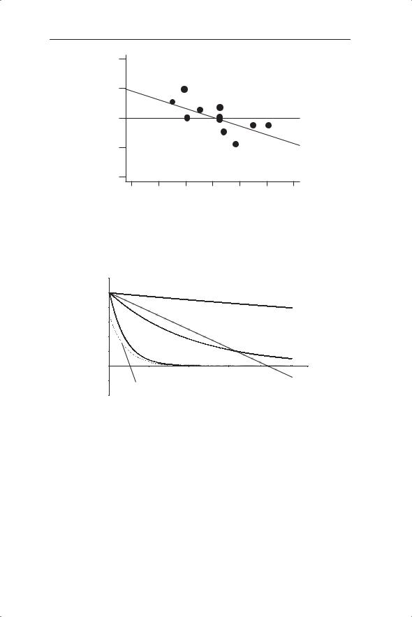
In the previous chapters we made some key simplifications concerning the dynamics of populations and clades. In particular, we assumed that under fluctuating environmental conditions the numbers of populations or lineages may drift continually upwards or downwards (until extinction) over time and that under constant conditions they may increase or decrease geometrically. Such continual drifting and/or geometric change is unrealistic under most conditions. Real populations often seem to be limited in their size and to be relatively abundant or relatively rare. The same may be true of clades in terms of the number of lineages. Populations that persist over long periods of time are presumed to be regulated in some way. The mechanism underlying this regulation is referred to as density-dependent change in survival or fecundity or, more succinctly, density dependence. For example, as the density of organisms increases there is an increase in the fraction of individuals dying (Fig. 5.1); that is, mortality is no longer constant for a particular age or stage of organism but is determined by the density of organisms (recall that density may refer to numbers or biomass per unit area or volume). Density dependence can be driven by processes such as competition or predation. For example, as population density increases, resources may become depleted and intraspecific competition become increasingly important, or predators may preferentially select prey at higher density. It is these assumptions of factors altering with population density that underlie the regulation of populations. Most ecologists agree that only density dependence can regulate populations. Later we will consider the extent to which clades may also show such density-dependent processes.
There are many examples of density dependence in the ecological literature (Fig. 5.1). These may be derived from laboratory or field experiments in which the density of organisms is altered (Figs 5.1a and 5.1b) or from natural variation in density in the field (Figs 5.1c and 5.1d).
An alternative to the detection of density dependence by experimentation is to examine the population dynamics for evidence of density dependence. The change in numbers from one time period (e.g. a year) to the next can be expressed as Nt+1/Nt or log Nt+1 − log Nt. This change is plotted against density
72

REGULATION IN TEMPORAL MODELS |
73 |
(a) |
(b) |
Egg density (arbitrary units) |
Egg density (arbitrary units) |
(c) |
(d) |
Fig. 5.1 Examples of survival and fecundity altering with population density in (a,b) Drosophila melanogaster (Prout & McChesney 1985) and (c, d) great tits (Parus major; data of Kluiver in Hutchinson 1978).
(Nt) to look for density dependence (Fig. 5.2). The null hypothesis is that there is no relationship between the change in population density and density itself. If density dependence is occurring then when density is low population size is likely to increase (Nt+1/Nt will be greater than 1) and when density is higher the population size is likely to decrease. Therefore we would expect a negative slope on a graph of change in population density against density under conditions of density dependence. The statistical significance of deviation from the null hypothesis of a gradient of 0 can be determined (although these analyses are problematic as we will see later). This method can also be applied within years to look for density-dependent survival or fecundity, both of which may contribute to a change in population numbers over time.
If we are to make our models more realistic then we must understand how density dependence affects population dynamics and incorporate it into these models.
5.2 Equations for modelling density dependence
The essence of density-dependent mechanisms for models of population dynamics is that, as the density increases, there is an alteration in the
74 CHAPTER 5
1
r2 = 0.42
P = 0.024
2
Rt 0
−1
−2
0 |
5 |
10 |
15 |
20 |
25 |
30 |
Xt-1
Fig. 5.2 Detection of density dependence by linear regression. In this example the population change in common sardine (Strangomera bentincki) from one year to the next (Rt = log Xt − log Xt−1) is regressed against its density in year t − 1 (Pedraza-Garcia & Cubillos 2008). Note that the use of t and t − 1 could be replaced by t + 1 and t.
|
1.2 |
|
|
|
|
|
|
1 |
|
|
|
s = e−0.01N |
|
(s) |
|
|
|
|
|
|
0.8 |
|
|
|
|
|
|
surviving |
|
|
|
|
|
|
0.6 |
|
|
s = −0.05N + 1 |
|
|
|
0.4 |
|
|
|
|
|
|
Fraction |
|
|
|
|
|
|
0.2 |
|
|
|
s = e−0.1N |
|
|
|
s = e−0.5x |
|
|
|
||
0 |
|
|
|
|
||
|
0 |
5 |
10 |
15 |
20 |
25 |
|
−0.2 |
s = 0.7e−0.5x |
|
|
|
|
|
|
|
|
|
|
|
|
−0.4 |
|
|
Density (N) |
|
|
|
|
|
|
|
|
Fig. 5.3 Exponential and linear decline in fraction surviving (s) with density (N). Notice the change in shape with increasing values of a (see text for details). The intercept of the exponentially declining function can be easily altered (dashed line).
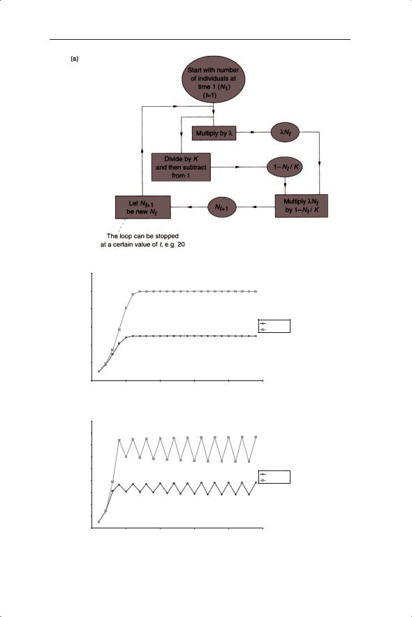
fecundity or fraction of individuals surviving and therefore a change in λ, the finite rate of population change. In open systems we can invoke densitydependent changes in migration, but these are not considered in this chapter. In Fig. 5.3 a set of lines have been drawn, illustrating some possible densitydependent functions (the vertical axis is labelled s to indicate the fraction surviving). In order to include these in population models we need to describe them in mathematical terms. For example, the linear decline in s with increasing density is expressed as the equation of a straight line:

REGULATION IN TEMPORAL MODELS |
75 |
s = c − mN |
(5.1) |
where c is the intercept on the vertical (s) axis and m is the magnitude of the gradient of the line. c must lie between 0 and +1 as we are considering the fraction surviving. Equation 5.1 tells us that at the lowest (non-zero) density the value of s is close to maximum (c) and that with increasing density the fraction of individuals surviving decreases linearly according to the gradient m. The linear reduction in s with N assumes that there is a density, Nmax, at which s = 0. In other words there is an upper (Nmax) and lower boundary (0) of possible extinction. If a population goes above Nmax it will become extinct. This upper boundary clearly creates some problems for modelling purposes. To overcome this we will consider a second mathematical function of exponential decline:
s = e−aN |
(5.2) |
The change in s with increasing values of N for three different values of a (0.5, 0.1 and 0.01) is shown in Fig. 5.3 (recall that equation 5.2 can be natural-log transformed to give ln(s) = −aN, showing that the natural log of s declines linearly with N). The parameter a can be thought of as denoting the strength of density dependence. At any given value of N, the fraction surviving will decrease as a increases. When N = 0, s will be equal to 1, regardless of the value of a; that is, the model is designed so that at very low densities s tends towards a maximum value. Conversely, at very high densities, the value of s tends towards 0 but never reaches it (an example of an asymptote) unlike the linear density dependence. The function can be altered to s = be−aN to give a maximum value different from 1 at N = 0.
Some of the different curves in Fig. 5.2 can be considered to represent different types of intraspecific competition. An important distinction is between scramble and contest competition (Hassell 1975). In pure scramble competition, resources are divided equally among competing individuals. The consequence of this is that above a certain density the mean resource per individual is too low for survival, and therefore s plummets to zero. The upper boundary in the discrete logistic model (Section 5.4) could be interpreted as representing perfect scramble competition. The other extreme is contest competition, in which the superior competitors monopolize the resource. Consequently, a certain number of individuals always survive, even at high densities. In this case, s would approach zero at high densities, but never reach it, in agreement with the exponentially declining curve.
5.3 A density-dependent model of population dynamics
Let us return to the annual plant model from Chapter 2 and consider how density dependence may be incorporated into that density-independent model. Imagine that competition for space occurs between juvenile and adult

76 CHAPTER 5
plants: that there is intraspecific competition. The effect of competition on individual survival is expected to increase as plant density increases. In years of low plant density there will be relatively high survival but increasing density will result in reduced survival. We have seen that the simplest model for density dependence is a linear change represented by s = −mN + c (equation 5.1). In the following example we will use d as the density of individuals subjected to density dependence. In the density-independent model we assumed that an average of 0.2 plants survived after germination up to seed set. In the new density-dependent model, 0.2 can be taken as the value of c; that is, when the effects of density are negligible. Therefore s is close to c at the lowest population densities and, with any increase in density, s declines linearly according to the gradient m. The linear reduction assumes that there is a density, dmax, at which s = 0, so that m = 0.2/ dmax (i.e. c/dmax). Therefore the linear density dependence equation can be written as s = 0.2 − (0.2/dmax)d or s = 0.2(1 − d/dmax). A new model, incorporating density dependence, now replaces the old density-independent model:
Number of germinating seed next year (Nt +1 ) = number of seed germinating this year (Nt ) × fraction surviving to seed set (0.2(1 − d dmax )) × average number of seeds produced (100) × fraction surviving over winter (0.1)
If the fecundity and survival values are combined, as before, into the single value, λ (=0.2 × 100 × 0.1), we produce the equation:
Nt +1 = Nt λ (1 − d dmax ) |
(5.3) |
In this case the interpretation of density dependence is that the fraction of germinating seed that survives is reduced by increasing density, which could be caused by intraspecific competition. In year t, d will be equal to 0.2Nt. If 0.2/dmax is replaced by 1/K we obtain:
Nt +1 = λNt(1 − Nt K ) |
(5.4) |
Equation 5.4, incorporating density dependence, is known as the discrete logistic equation and represents a strategic model for the population dynamics of annual species. K is the carrying capacity, defined as the maximum number of individuals a habitat can support. Equation 5.4 is sometimes written as Nt+1 = λNt(1 − αNt); that is, replacing 1/K by α. Berryman (1992) and Elliott (1994) review the use of the discrete logistic and similar equations whereas May et al. (1974) and May (1981) discuss the density-dependent terms.
Modelling of intraspecific competition has lead to a variety of equations incorporating density dependence. The model of Hassell (1975), described by the equation Nt+1 = λNt(1 + aNt)−b, provides parameters a and b which can describe change from contest to scramble competition. a gives the threshold

REGULATION IN TEMPORAL MODELS |
77 |
density at which density dependence occurs and b is the strength of the density dependence. This model, derived from earlier studies of insects (Morris 1959, Varley & Gradwell 1960), was related to models of fisheries (Nt+1 = λNt(1 + aNt)−1 (Beverton & Holt 1957). In turn, the model of Hassell was developed by Watkinson (1980) to describe the population dynamics of annual plants:
Nt +1 = λNt ((1 + aNt )b + wλNt )
where a and b are the parameters of the Hassell model, w is the degree of self thinning and λ is the finite rate of population change.
We will now consider some of the properties of equation 5.4 and compare them with the density-independent equations in Chapter 2. If we multiply out the right-hand side of equation 5.4 we see an important attribute of the density-dependent equation:
Nt +1 |
= λNt − (λNt2 |
K ) |
(5.5) |
|
|
|
|
Equation 5.5 clearly demonstrates that the discrete logistic is a nonlinear equation; in particular it is a quadratic equation, indicated by the presence of Nt2. Its full title is a first-order nonlinear difference equation. It is first order because it relates values at time t + 1 to the previous time points (t). A secondorder difference equation would relate values at time t + 1 to the previous two time points (t and t − 1). It is the non-linear component that gives this and similar equations (May 1976) some fascinating properties which we will now explore.
5.4 Exploration of the dynamics produced by the discrete logistic equation
We have two options in exploring the behaviour of equations such as the discrete logistic. First, given initial conditions, for example an initial number of germinating plants, and values for the parameters K and λ, we can generate a series of plant values as we did for the density-independent model. This is a simulation approach to the exploratory process: it will show us what the equation (model) can do but not necessarily tell us much about why it does it. If we want to know why, then we have to carry out some form of mathematical analysis, which is referred to as the analytical approach. Some analytical techniques are detailed after the simulations.
Values of N generated from simulations using equation 5.4 are displayed in Fig. 5.4. Starting with 10 germinating plants, Fig. 5.4a shows a flow diagram of the sequence of calculations in the simulation (such simulations can be written in widely available spreadsheet packages). This is an iterative process in which we generate a value for Nt+1 and then use it as the new Nt and so on. You should check the first few iteration values given in Fig. 5.4b.
78 CHAPTER 5
(b) |
|
|
|
|
|
|
|
120 |
|
|
|
|
|
|
100 |
|
|
|
|
|
density |
80 |
|
|
|
|
|
|
|
|
|
|
K = 100 |
|
Population |
60 |
|
|
|
|
|
|
|
|
|
K = 200 |
||
|
|
|
|
|
||
40 |
|
|
|
|
|
|
|
|
|
|
|
|
|
|
20 |
|
|
|
|
|
|
00 |
5 |
10 |
15 |
20 |
25 |
|
|
|
|
Time |
|
|
(c) |
|
|
|
|
|
|
|
180 |
|
|
|
|
|
|
160 |
|
|
|
|
|
density |
140 |
|
|
|
|
|
120 |
|
|
|
|
|
|
100 |
|
|
|
|
|
|
Population |
|
|
|
|
K = 100 |
|
80 |
|
|
|
|
||
|
|
|
|
K = 200 |
||
60 |
|
|
|
|
|
|
40 |
|
|
|
|
|
|
|
|
|
|
|
|
|
|
20 |
|
|
|
|
|
|
0 |
5 |
10 |
15 |
20 |
25 |
|
0 |
|||||
|
|
|
|
Time |
|
|
Fig. 5.4 (a) Flow diagram of the sequence of calculations showing how to generate successive values of Nt using the discrete logistic equation (equation 5.4). Change in density (Nt) with time generated from the discrete logistic equation with K = 100 and 200 and λ taking the values: (b) 2, (c) 3.1, (d) 3.5 and (e) 4. All graphs start with N1 = 10.
Continued
REGULATION IN TEMPORAL MODELS |
79 |
|
(d) |
|
|
|
|
|
|
|
|
200 |
|
|
|
|
|
|
|
180 |
|
|
|
|
|
|
density |
160 |
|
|
|
|
|
|
120 |
|
|
|
|
|
|
|
|
140 |
|
|
|
|
|
|
Population |
100 |
|
|
|
|
K = 100 |
|
|
|
|
|
K = 200 |
||
|
|
|
|
|
|
||
|
|
|
|
|
|
|
|
|
|
80 |
|
|
|
|
|
|
|
60 |
|
|
|
|
|
|
|
40 |
|
|
|
|
|
|
|
20 |
|
|
|
|
|
|
|
0 |
5 |
10 |
15 |
20 |
25 |
|
|
0 |
|||||
|
|
|
|
|
Time |
|
|
|
(e) |
|
|
|
|
|
|
|
|
250 |
|
|
|
|
|
|
density |
200 |
|
|
|
|
|
|
150 |
|
|
|
|
|
|
|
|
|
|
|
|
|
|
|
Population |
|
|
|
|
|
K = 100 |
|
100 |
|
|
|
|
K = 200 |
|
|
|
|
|
|
|
||
|
|
|
|
|
|
|
|
|
|
50 |
|
|
|
|
|
|
|
0 |
5 |
10 |
15 |
20 |
25 |
|
|
0 |
|||||
|
|
|
|
|
Time |
|
|
Fig. 5.4 |
Continued |
|
|
|
|
|
|
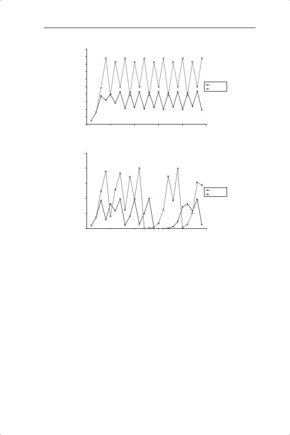
The dynamics of the model population over time at different values of λ can be summarized as follows. At λ = 2 the population approaches an equilibrium value of K/2 at which it remains (Fig 5.4b); that is, this appears to be a stable equilibrium value. Recall from Chapter 2 that the equilibrium is defined as the population density to which or around which a population will move, whereas stability describes the tendency of a population to stay at or move towards or around the equilibrium. We have seen that densityindependent dynamics can only produce a steady state if λ = 1. In contrast, density dependence allows an ecologically feasible stable equilibrium with different values of λ. At λ = 3.1 (Fig. 5.4c) the population oscillates between two densities; this is referred to as a two-point limit cycle. At λ = 3.5 (Fig. 5.4d) four-point limit cycles are produced whereas at λ = 4 (Fig. 5.4e) the initially regular cycles break up, so that the population fluctuates, apparently unpredictably, between a series of densities. This is referred to as chaotic dynamics: the mathematical definition of chaos and its importance in ecology

80 CHAPTER 5
is considered below. In this equation the values of K do not affect the dynamics and only contribute to the size of the equilibrium.
To be certain of the stability of the equilibrium with λ = 2 we need to displace the population from the assumed equilibrium and check its return. This can be achieved by running the model from different initial conditions and would show that the equilibrium of 50 is indeed stable; in fact it is globally stable for all ecologically realistic values. ‘Global stability’ has to be qualified to accommodate a flaw in the model, which is that it will crash if values of Nt exceed K (because 1 − Nt/K becomes negative). The two-point limit cycle is also stable; for a given value of λ (within the range of values giving twopoint cycles) the population will always settle out to fluctuate between the same two densities so that there are now two stable equilibriums. In contrast, the chaotic dynamics do not have this property. Here, the particular sequence of values is dependent upon initial conditions, although the size of the fluctuations will be determined by the values of λ and K.
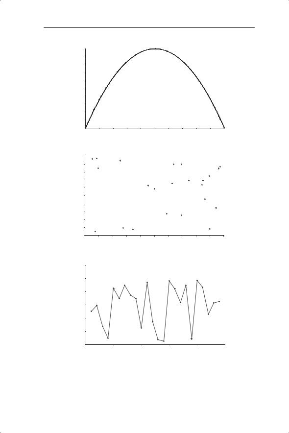
The possibility of chaotic dynamics means that if ‘random’ or unpredictable dynamics are recorded this does not necessarily imply that the underlying mechanisms are random (stochastic). Some or all of the ‘randomness’ could be produced by predictable deterministic processes expressed as chaos. Thus, if population change is described by the discrete logistic equation each population size at t + 1 (Nt+1) is given by a particular value of Nt. We can see this clearly by plotting Nt+1 against Nt (Fig. 5.5a) using the parameter values for λ and K of 4 and 100 (Fig. 5.4e). The chaotic system shows the mathematical relationship of the discrete logistic: a quadratic equation. A fit through the points gives (as expected) a perfect fit indicated by the r2 of 1. The coefficients of −0.04 and +4 agree with equation 5.5 (−λ/K for Nt2 and λ for Nt). This can be compared with a truly random sequence of values where Nt+1 plotted against Nt is a cloud of points (Fig. 5.5b).
The challenge of detecting chaos in real population dynamics is therefore to distinguish it from random events. The first study to try to detect chaos in laboratory and field populations was by Hassell et al. (1976). They used the technique of assuming an underlying mathematical model (described by the equation Nt+1 = λNt(1 + aNt)−b discussed above) and determining the values of λ, a and b for different populations of insects. They were then able to compare these values with those known to produce limit cycles and chaos (Fig. 5.6). So Hassell and colleagues were testing whether the model that is fitted to the data has parameter values which would give chaos. The parameter values of b and λ for each species were superimposed on the regions of different dynamic behaviour predicted by the model; for example, stable equilibrium, limit cycles and chaos.
Only one species had values consistent with chaotic dynamics and one consistent with limit cycles. All the other populations were in the stableequilibrium region. It is worth noting that the apparently chaotic population was a laboratory population of blowflies studied by Nicholson (1954). The
REGULATION IN TEMPORAL MODELS |
81 |
(a) |
|
|
|
|
|
|
|
|
|
|
|
|
|
100 |
|
|
|
|
|
|
|
|
|
|
|
|
90 |
|
|
|
|
|
|
|
|
|
|
|
) |
80 |
|
|
|
|
|
|
|
|
|
|
|
1 |
|
|
|
|
|
|
|
|
|
|
|
|
t+ |
|
|
|
|
|
|
|
|
|
|
|
|
|
|
|
|
|
|
|
|
|
|
|
|
|
(N |
70 |
|
|
|
|
N |
|
= −0.04N 2 |
+ 4N |
|
|
|
1 |
|
|
|
|
|
|
|
|
||||
|
|
|
|
|
t+1 |
t |
|
|
||||
t + |
60 |
|
|
|
|
|
t |
|
|
|
||
|
|
|
|
|
|
r2 = 1 |
|
|
|
|
||
at time |
50 |
|
|
|
|
|
|
|
|
|
|
|
40 |
|
|
|
|
|
|
|
|
|
|
|
|
Number |
|
|
|
|
|
|
|
|
|
|
|
|
30 |
|
|
|
|
|
|
|
|
|
|
|
|
20 |
|
|
|
|
|
|
|
|
|
|
|
|
|
10 |
|
|
|
|
|
|
|
|
|
|
|
|
0 |
10 |
20 |
30 |
40 |
50 |
60 |
70 |
80 |
90 |
100 |
|
|
0 |
|||||||||||
(b) |
|
|
|
Number at time t (Nt) |
|
|
|
|
||||
|
|
|
|
|
|
|
|
|
|
|
||
|
100 |
|
|
|
|
|
|
|
|
|
|
|
|
90 |
|
|
|
|
|
|
|
|
|
|
|
) |
|
|
|
|
|
|
|
|
|
|
|
|
t+1 |
80 |
|
|
|
|
|
|
|
|
|
|
1 (N |
70 |
|
|
|
|
|
|
|
|
|
|
t + |
60 |
|
|
|
|
|
|
|
|
|
|
time |
|
|
|
|
|
|
|
|
|
|
|
50 |
|
|
|
|
|
|
|
|
|
|
|
at |
40 |
|
|
|
|
|
|
|
|
|
|
Number |
|
|
|
|
|
|
|
|
|
|
|
30 |
|
|
|
|
|
|
|
|
|
|
|
20 |
|
|
|
|
|
|
|
|
|
|
|
|
|
|
|
|
|
|
|
|
|
|
|
|
10 |
|
|
|
|
|
|
|
|
|
|
|
0 |
10 |
20 |
30 |
40 |
50 |
60 |
70 |
80 |
90 |
100 |
|
0 |
||||||||||
|
|
|
|
|
Number at time t (Nt) |
|
|
|
|||
(c) |
|
|
|
|
|
|
|
|
|
|
|
|
120 |
|
|
|
|
|
|
|
|
|
|
|
100 |
|
|
|
|
|
|
|
|
|
|
density |
80 |
|
|
|
|
|
|
|
|
|
|
|
|
|
|
|
|
|
|
|
|
|
|
Population |
60 |
|
|
|
|
|
|
|
|
|
|
40 |
|
|
|
|
|
|
|
|
|
|
|
|
|
|
|
|
|
|
|
|
|
|
|
|
20 |
|
|
|
|
|
|
|
|
|
|
|
0 |
|
5 |
|
10 |
|
15 |
|
20 |
|
25 |
|
0 |
|
|
|
|
|
|||||
|
|
|
|
|
|
Time |
|
|
|
|
|
Fig. 5.5 Nt+1 plotted against Nt for (a) chaotic and (b) random time series (the time series is shown in (c)). The chaotic time series is given in Fig. 5.4e.