1gillman_m_an_introduction_to_mathematical_models_in_ecology

102 CHAPTER 6

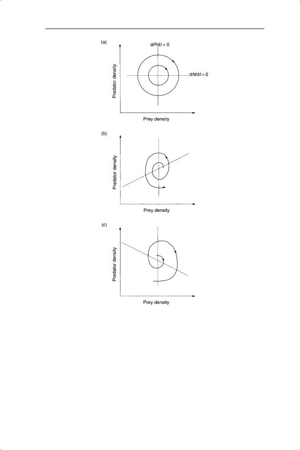
Fig. 6.5 An example of a plot of the trajectory of predator and prey dynamics on a phase plane.

If the dP/dt = 0 line is kept vertical and the slope of dN/dt = 0 is altered, what is the effect on dynamics and stability? In particular, what happens when dN/dt = 0 is horizontal, which is equivalent to removing the prey density dependence? In this case, starting at any point simply sends the trajectory on an elliptical path back to where it started (Fig. 6.6a). This is an example of neutral stability, for which the Lotka–Volterra model received much criticism. Neutral stability, akin to a frictionless pendulum, is referred to as a structurally unstable model (May 1973a), in which the amplitude of cycles is determined by initial conditions and the cycles persist with unchanging amplitude. This is in contrast to the limit cycles in Chapter 5 where the cycles fluctuate between particular densities regardless of the initial conditions; that is, the starting density. If the gradient of dN/dt = 0 is positive then the trajectory spirals out leading to unrealistically high values of predator and prey (Fig. 6.6b). When the gradient of dN/dt is negative, as in the above example, the result will be a stable equilibrium (Fig. 6.6c).

In fact, with the Lotka–Volterra equations, the only cycles produced are neutrally stable. Although Volterra considered the possibility of using equation 6.2 in his predator–prey model, noting that the fluctuations would be damped and the system would tend towards the stationary state, he did not pursue this line of enquiry. Most of his emphasis in predator–prey systems was on the possibility of cycles using equation 6.3 without prey regulation and equation 6.4. For structurally stable cycles we need a time delay of some description, which may be expressed either as a delay differential equation (Hutchinson 1948) or, as in the next section, by coupled difference equations.

Fig. 6.6 Effect of changing the gradient of dN/dt = 0 on stability in Lotka–Volterra models. (a) Neutrally stable cycles of predators and prey (gradient of dN/dt = 0).

(b)Densities of predators and prey spiral out (gradient of dN/dt = 0 is positive).

(c)Densities of predators and prey spiral into a stable equilibrium (gradient of dN/dt = 0 is negative). Reprinted from Maynard Smith (1974).

6.2.3 Explaining cycles of abundance with models in discrete time

We will now consider a discrete version of the Lotka–Volterra model (May 1973b) and then generalize this to a new type of equation. By analogy with equations 6.3 and 6.4:

Therefore, in the absence of predation the prey are self-regulated according to the discrete logistic (equation 6.5, with the finite rate of prey population change given by λN), and in the absence of prey the predators decline at the rate of λP (if it is assigned a value less than 1). If the time subscript for the predator equation 6.6 is reduced on both sides by 1:

Pt = λP Pt −1 + bPt −1Nt −1

and the right-hand side substituted for Pt in equation 6.5:

then we are left with a second-order nonlinear difference equation. The equation is second order because Nt+1 is explained by terms which are two time steps (Pt−1 and Nt−1) earlier, along with a term one time step earlier, Nt.

Therefore, a pair of coupled first-order difference equations is equivalent to a second-order difference equation. The dynamics produced by secondorder nonlinear difference equations are very interesting and quite different from their first-order cousins. Second-order equations can produce cycles which are similar to those of predators and prey observed in the field. To test this type of model we need to know a little more about the mechanisms underpinning predator–prey interactions.

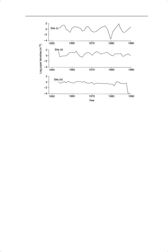
As an example consider the dynamics of the larch bud-moth (Zeiraphera diniana), which periodically defoliates its host tree, larch (Larix decidua), and the pine looper moth (Bupalus piniaria), which specializes on Scots pine (Pinus sylvestris). Detailed sampling of the larvae of the larch bud-moth has shown that the optimum area for survival and fecundity is the subalpine region of the Swiss Alps between 1700 and 2000 m (Baltensweiler 1993). In this region the larch bud-moth reaches carrying capacity within four or five generations and has cycle lengths of 8–9 years (Fig. 6.1). The clear cycles of Zeiraphera are in contrast to the rather irregular and sometimes absent cycles of Bupalus (Fig. 6.7).

Larch bud-moth cycles are an example of a herbivore population cycle explained by density-dependent changes in their food which may be modified by climate conditions. As larval densities increase, defoliation of the larch affects its physiology, reducing the quality and quantity (needle length) of the herbivore’s food that, in turn, triggers the collapse of the herbivore populations in the following years. Alteration in the plant (food) quality includes decreased nitrogen content and greater fibre content. This explanation of cycles has been contested by some ecologists, who claim that interactions between herbivores and their natural enemies generate the cycles. Note that forest trees, as prey, may fluctuate or cycle in the abundance of biomass or components such as nitrogen, rather than numbers.

Fig. 6.7 Cycles of population abundance of pine looper (Bupalus piniaria) at three sites.

The larch bud moth example is a clear case of delayed density dependence in which the effects of density dependence are carried over to the next generation via an interaction with the host plant. Delayed density dependence, first described by Varley (1947), underpins the dynamics of many predator– prey systems and can be described by second-order nonlinear difference equations. Broekhuizen et al. (1993) identified a delayed density-dependent mechanism by which population cycles may be produced in the pine looper moth, detailed below.

There is a strong negative correlation between annual growth increment of Pinus sylvestris in Tentsmuir forest and the pupal density of Bupalus piniaria in the previous two years (Straw 1991). This indicates that B. piniaria may have a substantial influence upon their host trees’ physiologies. This may ‘feed back’ upon the B. piniaria population such that the one year’s B. piniaria [population] influence the reproductive success of the next year’s population.

To explore models of delayed density dependence we will consider a secondorder nonlinear difference equation which can be parameterized from census data. This covers the work of Turchin (1990; see also Turchin & Taylor 1992) who used a second-order Ricker equation to investigate the likelihood of delayed density dependence among herbivorous forest insects, including Zeiraphera and Bupalus. We met the first-order version of the Ricker equation in Chapter 5 and will use the same regression technique to estimate parameters. The second-order version is:

106 CHAPTER 6

The parameters a and b represent the strength of direct and delayed density dependence respectively. Note that the right-hand side of equation 6.8 is equivalent to λNte(aNt+bNt−1). If b = 0 then equation 6.8 reverts back to the firstorder equation. For regression purposes we also assume an unexplained variance term in the model. To estimate the parameters a and b in equation 6.8 we divide by Nt and take natural logs:

ln (Nt+1/Nt) can then be regressed against Nt and Nt−1. This was the method used by Turchin (1990), who showed significant delayed density dependence (i.e. values of b significantly different from 0) in 10 out of 14 data sets. In considering the significance of the parameters we should recall the possibility of overestimating the significance of a or b using this regression model. The values of a, b and r for Bupalus and Zeiraphera are given in Table 6.1.

The dynamics resulting from the estimated parameter values can be found by simulation using equation 6.8 (Fig. 6.8). You will see that the predicted dynamics for the two species are quite different, with Bupalus predicted to be stable with an equilibrium population size of about 150. Zeiraphera, in contrast, is predicted to cycle with periods of 6–7 years, slightly shorter than the 8–9 year cycles observed in the field. These results are in agreement with the clearly defined cycles of Zeiraphera and poorly defined cycles of Bupalus. Analysis of equation 6.9 therefore suggests a much stronger deterministic signal for cycle production in Zeiraphera compared with Bupalus.

Simulation of another second-order model in Broekhuizen et al. (1993) also suggests a stable equilibrium for Bupalus populations. The critical parameter determining cyclical behaviour in equation 6.8 is r. Indeed, whereas 10 out of 14 of Turchin’s data sets showed delayed density dependence, only three have values of r high enough to produce cycles. Turchin and Taylor (1992) noted that focusing on direct density dependence rather than delayed density dependence leads to potentially misleading results. They gave the example of the analysis of Hassell et al. (1976), who estimated density dependence and then looked at the stability (or otherwise) of insect population

Table 6.1 Parameter values derived from regression of equation 6.9 (Turchin 1990). Both values of a and b are significantly different from 0. Variance (%) is the percentage of variance in the dependent variable explained by variance in the independent variable (recall that this is a measure of goodness of fit of the regression and written as r2; not to be confused with the r in column 2, which is the intrinsic rate of change).

Fig. 6.8 Predicted dynamics of (a) Bupalus and (b) Zeiraphera using equation 6.8 and the parameter values in Table 6.1. The figure for Bupalus shows the population moving smoothly (and sigmoidally) from initial conditions of N1 = 10 and N2 = 10 towards a stable equilibrium. The figure for Zeiraphera is shown once the population has settled down from its initial conditions.

dynamics (Chapter 5). Hassell et al. classified the larch bud-moth in the Engadine Valley, Switzerland, as stable, although this population, was, according to Turchin and Taylor ‘arguably the most convincing example of a . . . cyclical system in our data set’. For further insights into the mechanisms underpinning cyclical and other population dynamics see Turchin (2003).

6.3 Competition models

In Chapter 5 we considered the possibility of intraspecific competition as a mechanism producing density dependence. In this chapter our attention is on competition between species, or interspecific competition. This will serve

108 CHAPTER 6

as a prelude to a generalized description of interactions between species in Chapter 7.

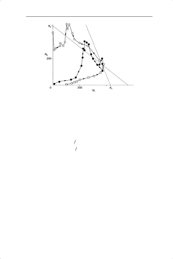
Much of the classic work on interspecific competition involved insects and micro-organisms including beetles in stored grain (Crombie 1945, 1946, 1947, Park et al. 1964), aquatic protozoa (Gause 1934, 1935) and yeast (Gause 1932, 1934). For example, the experiments of Crombie (1945, 1946) showed how three combinations of the beetles Tribolium confusum and Oryzaephilus surinamensis converged to the same population equilibrium. The beetles were fed on wheat, presented as either cracked grain or flour. In cracked wheat each species cultured in isolation increased to between 420– 450 adults in 150 days (represented as carrying capacities K1 and K2 in Table 6.2). The change in numbers over time is plotted on the phase plane in Fig. 6.9. However, when the species were combined, Tribolium reached 360 individuals and Oryzaephilus 150 individuals; thus the total was greater than the species in monoculture (represented as N1* and N2* in Table 6.2). The results were independent of the initial number of beetles, indicating that this was a globally stable equilibrium. As Pontin (1982) noted, ‘the total number of beetles in mixed culture at equilibrium is equal to or greater than the carrying capacity number of either (species) alone so the combination may be more efficient at converting grain to beetles.’ Changing the medium from flour grains to fine flour resulted in the extinction of Oryzaephilus. Small pieces of tubing which provided shelter for Oryzaephilus allowed the latter to survive under fine-flour conditions (Table 6.2). The same general effects of habitat structure on coexistence were found in the predator–prey experiments of Huffaker (1958).

Tribolium individuals are carnivorous: the larvae and adults eat eggs and pupae of their own species and also those of Oryzaephilus. Adult Oryzaephilus also consume Tribolium eggs but at a lower rate than its own are consumed by Tribolium. Therefore this interaction is part predation and part competition for resource. This emphasizes the need for a generalized model in which a variety of interactions are encompassed.

Table 6.2 Values of carrying capacity of Tribolium confusum (species 1) and Oryzaephilus surinamensis (species 2) in isolation (K1 and K2) and at equilibrium in mixtures (N1* and N2*) estimated from experiments. Values for the competition coefficients (β12, β21) are derived in the text (data in Pontin 1982 from Crombie 1946).

Fig. 6.9 Population trajectories from three competition experiments started with different numbers of Tribolium (N1) and Oryzaephilus (N2) in cracked-wheat cultures. The lines represent zero-growth isoclines of each species (from Crombie 1946, reprinted in Pontin 1982).

A pair of competing species such as Tribolium and Oryzaephilus can be described by a pair of simultaneous nonlinear differential equations similar to those used for the predator–prey interactions by Lotka and Volterra and, indeed, developed by Volterra (1926, 1928) and Gause (1934):

where N1 and N2 are the densities of the competing species. β12 describes the fraction of species 1 converted into species 2. This is known as the competition coefficient and is generalized to interactions between species i and j as βij. r is the intrinsic rate of change for a given species and K1 and K2 are the carrying capacities of species 1 and 2 in isolation. Note that equation 6.10 could also be written as:

dN1dt = r1N1((K1 − (N1 + β12N2 ))K1

As β12 is the fraction of species 1 converted to species 2 then N1 + β12N2 is effectively the density of N1, replacing N1 in the ordinary logistic equation (Chapter 5).

Investigation of stability with the phase plane begins, as with the predator–prey system, with the zero-growth isoclines (dN1/dt = 0 and dN2/ dt = 0). We will go through this more rapidly than the predator–prey example as many of the principles are the same. If we take the example of Tribolium and Oryzaephilus we find the values of K1, K2 and N1* and N2* (the equilibrium

110 CHAPTER 6

densities in mixtures) from the experiment (Table 6.2). With zero growth, equations 6.10 and 6.11 are:

K1 − N1* − β12N2* = 0, which gives N1* = K1 − β12N2*. Similarly, equation 6.13 yields N2* = K2 − β21N1*. As the values of N1*, N2*, K1 and K2 are known we can use these equations to find β12 and β21 and plot the zero-growth lines (Figs 6.9 and 6.10).

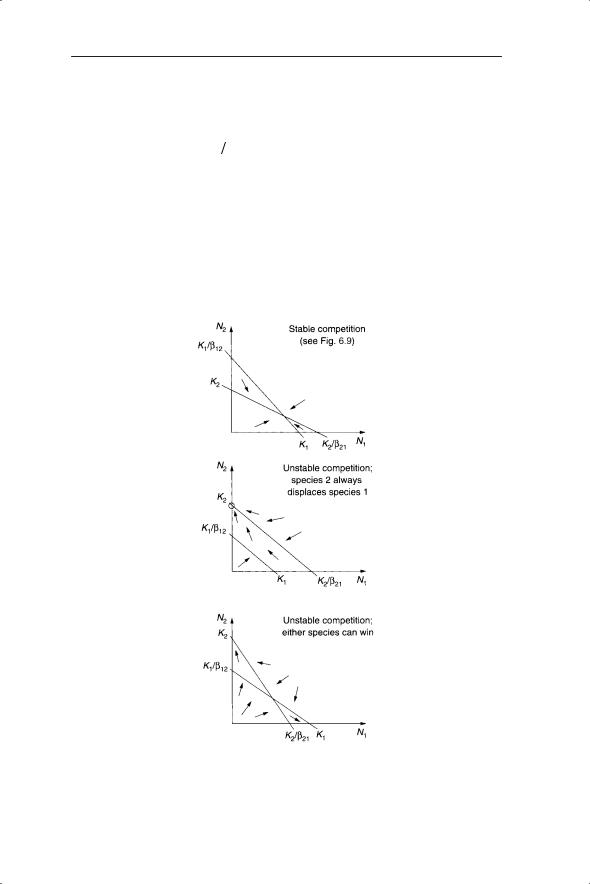
The outcomes of competition can now be investigated on the phase plane in the same way as for predator–prey interactions. These outcomes are (i) stable competition in which both species coexist, (ii) unstable competition in

Fig. 6.10 Three outcomes of interspecific competition based on three combinations of zero growth isoclines from equations 6.12 and 6.13.

which one species always displaces the second species – that is, there is a fixed hierarchy of competition – and (iii) unstable competition in which either species can win (Fig. 6.10). The assessment of competition coefficients in the field is developed in the context of generalized Lotka–Volterra models in Chapter 7. Another interesting development is the use of Lotka–Volterra competition models in combination with Markov models (Spencer & Tanner 2008)

Other competition models have been developed using discrete-time versions of equations 6.10 and 6.11; for example, the model of Hassell and Comins (1976):

N1,t +1 = λ1N1,t(1 + a1(N1,t + β1N2,t ))−b1

N2,t +1 = λ2N2,t(1 + a2(N2,t + β2N1,t ))−b2

β1 and β2 are the competition coefficients, a1 and a2 give the threshold densities at which density dependence begins and b1 and b2 are parameters that describe the different types of intraspecific competition, with extremes of scramble and contest (see Chapter 5 for discussion of the one-species analogue of this model). λ is the finite rate of population change for each species. Atkinson and Shorrocks (1981) used the model of Hassell and Comins to explore the effect of aggregation of competing Drosophila species on coexistence. The degree of aggregation was modelled using the negative binomial distribution. An increased aggregation of the superior competitor promoted coexistence. The importance of aggregation is highlighted in the next section with respect to host–parasitoid models.

6.4 Models of host–parasitoid interactions

Although delayed density dependence may arise due to interactions between herbivores and plant (section 6.2) this does not mean that interactions with the food plant are always the reason for the cycles in herbivores. Delayed density dependence may also occur due to interactions between a herbivore and its natural enemies; for example, parasitoids. Parasitoids are primarily wasps which lay their eggs on or inside a host larva, such as a moth or a fly. Indeed, Varley originally coined the term delayed density dependence because of his work on the parasitoids of the herbivorous fly, Urophora jaceana, which feeds on black knapweed, Centaurea nigra.

It has been estimated that more than 10% of all metazoan animals are parasitoids (Hassell & Godfray 1992) so it is important to understand how parasitoids interact with their hosts and, in particular, the type of dynamics which may be produced. Certain characteristics of parasitoid behaviour and life history may affect their dynamic interaction with their hosts (usually herbivorous insects, although there are parasitoids of parasitoids called