1gillman_m_an_introduction_to_mathematical_models_in_ecology

62 CHAPTER 4

equations. Alternatively we can employ analytical techniques, in which case it is helpful to rewrite the equations in a different form, employing a matrix structure. As we do so, you might wish to consider whether you expect any fundamental differences in the dynamics of this population to the one described by equation 2.2.

Equations 4.2 to 4.6 can be represented as three matrices:

Three matrices are required to summarize the five difference equations. There are two column matrices representing the number of individuals at ages 1–5 at times t + 1 and t (vt+1 and vt respectively). These column matrices are referred to as the population-structure vectors or age-distribution vectors. There is also one square matrix, M, which gives all of the fecundity and survival values and is known as the population projection matrix. To check that equation 4.7 is equivalent to equations 4.2–4.6 you can multiply out the matrix and population-structure vector on the right-hand side of the equation. For readers unfamiliar with matrix multiplication, you begin by multiplying the five coefficients in the top row of the square matrix M by the corresponding population sizes in the column matrix vt (0 × N1, 0 × N2, s0,1f3 × N3 and so on) and add the resulting five multiplied pairs of values to give N1 in vt+1. This process is then repeated with the next row, again multiplying by the corresponding values of N1–N5 in vt and summing the five multiples. This process is repeated for all five rows of the matrix M. Representation of age-structured populations in this manner was first described by Bernardelli (1941), Lewis (1942) and Leslie (1945, 1948).

Matrix equations such as equation 4.7, representing a set of difference equations, can be written in a general form to describe any ageor stage- structured population:

where vt and vt+1 are population vectors of the numbers of individuals at different ages (or sizes or stages) at t and t + 1 respectively, and M is a square matrix in which the number of columns and rows is equal to the number of age classes. You will see the similarity of this to equation 2.2, Nt+1 = λNt. This similarity is considered in the next section as we proceed with an analytical study of the dynamics of equation 4.8.

4.2 Determination of the eigenvalue and eigenvector

To proceed with the analytical investigation we will take a much simpler age-structured population and then discuss more complicated examples in the light of results from the simpler version. Consider a population of biennial plants (Fig. 4.2). The plant population has two age classes, which correspond to particular developmental stages. In the first year the plant forms rosettes following the germination of over-wintering seed. In the second year the surviving rosettes flower, set seed and then die. We will assume that the plant is a strict biennial: it always flowers in the second year (assuming it survives) and always dies after flowering. This model could also be described as a stage-structured population (Lefkovitch 1965; see Manly 1990 for an overview of matrix models of stage-structured populations) composed of rosettes and flowering plants. It is a coincidence in this case that each stage survives for one unit of time: in most cases this would not be true; for example, a tree species may spend many years at one defined stage. The dynamics of the population can be summarized with two first-order equations:

where R is the number or density of rosette plants, F is the number of flowering plants, f is the average number of viable seed per flowering plant, s0,1 represents the fraction of seed surviving between dispersal from the mother plant to rosette formation and s1,2 describes the fraction of rosettes surviving until flowering.

In constructing such models it is often the case that stages such as seed are omitted. This will depend on the units of time chosen for the model and the census time. For example, we could have examined changes from spring to autumn and autumn to spring in which case seed may need to be included as a specified stage, or at least a seed/small rosette stage.

Fig. 4.2 Representation of the life cycle of a biennial plant species with fecundity (f) and survival at two different stages (s0,1 and s1,2). Seed as a separate stage is not included in this model.

We are now left with a quadratic equation (4.17). Initially this poses a problem because a quadratic equation has two solutions (or roots); in other words, λ can have two values. But earlier we had assumed that the square matrix M could be replaced by a single value, λ. Effectively this becomes true as the larges of the two λ values, referred to as the dominant root, has most influence on the dynamics. Note that the dominant root may be complex or negative. A negative dominant root is biologically meaningless in this application (but see Chapter 7) whereas complex roots are discussed in Chapter 7. In mathematics the values of λ are called the eigenvalues and the corresponding values of R and F are the eigenvectors. The eigenvalues may also be referred to as the latent roots or the characteristic values of the matrix, M. Similarly, the eigenvectors are known as the latent or characteristic vectors. (In passing it is worth noting that in finding values for R and F we have found solutions for the equations 4.9 and 4.10. Matrix methods have a wide application in the solving of simultaneous equations.) Finally, it may be helpful to know that equations 4.13–4.16 can be written in a general mathematical shorthand for any size of matrix M and vector v (as equation 4.8):

Mvt = λvt

Mvt − λIvt = 0 (M − λI)vt = 0

The requirement for the non-trivial solution is that

M − λI = 0

with values of λ being found by solution of the characteristic equation.

To reinforce all these theoretical points let us consider a specific example. If f = 100, s0,1 = 0.1 and s1,2 = 0.5 then from equation 4.17:

λ2 = 100 × 0.1 × 0.5

λ2 = 5

λ= ± 5

+5 is both the larger value (and therefore the dominant root) and the one which is ecologically meaningful. We can now use this value of λ to produce

a prediction of the rate of increase of R and F (based on equation 4.12):

vt +1 = 5vt

or

Time (years)

Fig. 4.3 Simulation of population dynamics of rosettes and flowering plants (equations 4.9 and 4.10) with values of f = 100, s0,1 = 0.1 and s1,2 = 0.5.

It is important to note that the model predicts that both R and F increase at the same rate of 5 , and therefore predicts that they maintain the same ratio of R to F over time; that is, that they maintain a stable age structure. A quirk of this model is that it produces oscillations from year to year (Fig. 4.3). The yearly increase by 5 (λ) therefore needs to be viewed over a 2-year period; for example, from years 4 to 6 the rosette numbers increase 5-fold from 500 to 2500, equivalent to two yearly increases ( 5 × 5 ).

We can quantify the eigenvector and therefore determine the ratio of R to F as follows, using equation 4.13:

In effect we now have two equations: 10F = 5R and 0.5R = 5F. These two equations are equivalent because rearrangement of either produces

R = 2 5F.

68 CHAPTER 4

We have now achieved both parts of the analysis described at the beginning of this section: we have found a value for λ, the finite rate of change, by determining the eigenvalue of the matrix and we have calculated the ratio of R to F by quantifying the eigenvector.

These techniques can be applied to more complex examples in which there are more than two ages, stages or sizes of organisms. The number of eigenvalues is equivalent to the number of rows or columns and therefore the number of ages, stages or sizes in the projection matrix M. Although the determination of eigenvalues becomes more difficult as the matrix increases in size, the principle continues to hold that it is the dominant eigenvalue that is important. However large the projection matrix is, it can always be reduced to the dominant eigenvalue to describe the dynamics of the component stages of the population. Furthermore, the assumption of a stable age structure continues, given by the values in the eigenvector. Although we have focused on an age-structured population, it should be noted that many of the details of construction and results of the model are also relevant to stageor sizestructured populations.

The modelling of structured populations can be progressed by investigating the contributions of the various survival and fecundity values to the overall rate of change summarized by the eigenvalue (λ). These analyses have applications in harvesting and conservation of populations (Caswell 2000b). Sensitivity and elasticity are two related methods for determining contributions to the change in λ. Sensitivity quantifies the absolute changes in λ while elasticity quantifies relative changes in λ in response to proportional changes in elements of the projection matrix (de Kroon et al. 2000). Because the elasticity values sum to 1 the different components of the projection or transition matrix, such as the fecundity values, can be contrasted to show their importance to λ. This property has been used in comparative studies of life history across different taxa (e.g. Franco & Silvertown 2004).

4.3 Stochastic matrix models and succession

In Chapter 3 we saw how deterministic models of the form Nt+1 = λNt introduced in Chapter 2 can be developed by incorporating stochastic processes. Similarly, the deterministic matrix models outlined above have a stochastic counterpart (Fieberg & Ellner 2001) in which the various components of the matrix fluctuate in response to environmental change. These fluctuations are usually assumed to be like those of the random-walk example in Chapter 3; that is, independent and drawn from the same probability distribution. This type of process is referred to as a Markov process or Markov chain. The precise probability distribution used may vary within a given matrix or the probability distribution may be the same but the size of fluctuation may vary. There is also the possibility of including a deterministic signal. Fieberg and

Table 4.1 Fifty-year tree-by-tree transition matrix for grey birch, blackgum, red maple and beech. Each value is a transition probability.

Ellner (2001) discuss the ways in which stochastic matrix models can be used to estimate population extinction parameters.

Succession is the directional change in plant and animal species over time in a particular area. Mathematical models of this phenomenon have represented it as a Markov chain (Horn 1975, 1981). This involves determining the probability that a given plant (or other species or suite of species) will be replaced in a specified time by another individual(s) of the same or different species. Under Markov chain assumptions these replacement probabilities do not change with time. At each point in time, the relative abundances of species are multiplied by the transition probabilities to generate new relative abundances. This is iterated over a given number of time intervals. For example, Horn (1975, 1981) gave the values for 50 year tree-by-tree replacement between four species (Table 4.1). The model can be represented in matrix form:

vt +1 Transition probability matrix vt

These models predict a stationary end point; that is, that there will be a fixed ratio of grey birch to blackgum to red maple to beech. This is analogous to the result of a stable age structure in a population model. Interactions over different periods of time and the end point of the Horn example are given in Table 4.2. The predicted end-point is compared with the observed composition in old growth forest.

Other studies have looked at successional transitions between woodland and other types of vegetation. For example, Callaway and Davis (1993) used aerial photographs to measure transition rates between grassland, coastal sage scrub, chaparral and oak woodland and their relationship to burning

70 CHAPTER 4

Table 4.2 Predicted composition of a succession at different time points.

Table 4.3 The percentage of vegetation type from aerial photographs in 1947 and 1989 in central coastal California.

Fig. 4.4 Annual transition rates among plant communities in (a) burned plots (n = 53) and (b) unburned plots (n = 78) as determined from changes in vegetation between 1947 and 1989 shown on aerial photographs. The numbers in the boxes represent the probabilities that a given community will stay the same (from year to year) whereas the numbers on the arrows estimate the probability that a community will change in the indicated direction.

and grazing in Gaviota State Park in central coastal California, USA, between 1947 and 1989. The percentages of vegetation (community) types in 1947 and 1989 are given in Table 4.3 based on 0.25 ha plots sampled from aerial photographs.

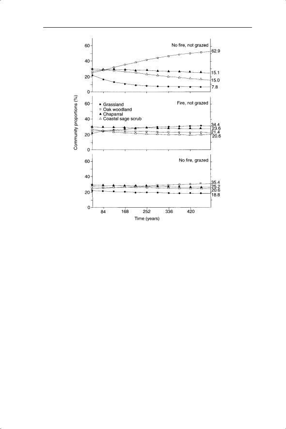
Fig. 4.5 Markov chain model predictions of future change in proportions of plant communities. Final community proportions at the end point (defined as <0.1% change over 42 years) are presented at the right, opposite each curve.

Although the overall percentage cover was very similar there was considerable flux between the years within plots. Transitions between vegetation type occurred in 71 out of 220 plots (32%). The transition probabilities were determined using these data (Fig. 4.4).

The current state could then be repeatedly multiplied by the four transitions (including no change) in the 42 year period to generate a Markov chain of predicted change in vegetation under particular environmental conditions. The predictions for three combinations of burning and grazing are given in Fig. 4.5.

Markov models are important tools in understanding landscape change and management. Modellers are using these tools in conjunction with statistical methods to assess spatial heterogeneity and rapidly improving data sets to provide more accurate predictions of primary and secondary succession (for example, Pueyo & Begueria 2007).