

1gillman_m_an_introduction_to_mathematical_models_in_ecology
.pdf112 CHAPTER 6
hyperparasitoids) including (i) searching area of the female parasitoid and (ii) interactions between female parasitoids.
The earliest model of host–parasitoid interactions was constructed by Nicholson and Bailey (1935). Their model was important as it made the case for time delays rather than the continuous time Lotka–Volterra equations described above. The main assumptions of their model are given below and illustrated in Fig. 6.11.
1Either zero or one parasitoid is produced per host (even if more than one egg is laid on a host).
2Each female parasitoid searches an area a, finding all the hosts. Therefore
the probability of a host being attacked is a/A where A is the total area and the probability of not being parasitized is 1 − a/A. If P is the density of para-
sitoids and A is the total area then there are AP female parasitoids. If para-
sitoids search independently and at random then the probability of a host not being attacked by any parasitoid is (1 − a/A)AP. If a/A is replaced by α
(defined as the proportion of total hosts encountered by one parasitoid per unit time) then we have (1 − α)AP which is equal to e−αP, the first term of the
Female searching area, a
Total area, A
Host larva
 Female parasitoid find all hosts in area a
Density of parasitoids |
A fraction (e-aP) |
|
P x area A = |
||
of larvae escape |
||
AP individuals |
||
|
Area A
Fig. 6.11 Summary of the assumptions of the Nicholson–Bailey model.

MODELLING INTERACTIONS |
113 |
Poisson distribution; that is, the probability of the host not containing parasitoids. The probability of being attacked at least once is then 1 − (probability of not being attacked), or 1 − e−αP.
3 The finite rate of increase of hosts (λH, in the absence of parasitoids) and parasitoids (λP) and the density of hosts (H) are known.
Using the above reasoning and assumptions Nicholson and Bailey produced a set of two equations in discrete time, one for the dynamics of the host (H) and one for the dynamics of the parasitoid (P):
Pt +1 = λP Ht(1 − e−αPt ) |
(6.14) |
Ht +1 = λHht e−αPt |
(6.15) |
Thus the number of parasitoids at time t + 1 (Pt+1) is equal to the number of hosts at time t (Ht) multiplied by the fraction of hosts which are attacked (1 − e−αPt) multiplied by the finite rate of increase of the parasitoids (λP); whereas the number of hosts at t + 1 (Ht+1) is equal to the number of hosts at t (Ht) multiplied by the fraction of hosts which are not attacked (e−αP) multiplied by the finite rate of increase of the host (λH).
The dynamics produced by these two equations have an unstable equilibrium and therefore produce cycles which can very easily become divergent (Fig. 6.12a) and lead to the local extinction of the parasitoid.
One option to stabilize the host populations is to introduce host (prey) density dependence. Host stability can be achieved by multiplying the finite rate of increase of the host (λH) by a linear term 1 − Ht/K, which can represent intraspecific competition among hosts. Beddington et al. (1975) examined the effect of including host density-dependent regulation. Stability was indeed much more likely and new types of dynamics were produced, such as five and 20 point cycles. This was compared with the host equation in the absence of predation which followed the standard period-doubling route to chaos (Chapter 5).
Other possibilities exist for stabilizing the host–parasitoid system; for example, the two assumptions of fixed search area and random searching by parasitoids have been shown to be unrealistic and to affect the stability of the interaction (Hassell & Godfray 1992). The effect of search area on stability was demonstrated by assuming competition between the parasitoids (Hassell & Varley 1969, Hassell & May 1973), which produces cycles or a stable equilibrium dependent on the intensity of interference (Fig. 6.12b). The effect of an aggregated distribution of parasitoids on host–parasitoid stability has been modelled using the negative binomial (May 1978). This will also produce a stable equilibrium or cycles dependent on the degree of aggregation.
The latter is an example of positive spatial density dependence in which, at one point in time, densities of hosts are spatially variable and high host densities receive an increased rate of parasitism. The density dependence discussed in previous chapters was temporal density dependence where

114 CHAPTER 6
Fig. 6.12 Dynamics of host and parasitoid (a) without density-dependent regulation of host or parasitoid. Observed fluctuations from an interaction between the greenhouse whitefly, Trialeurodes vaporariorum (closed circles) and a parasitoid wasp Encarsia formosa (open circles). Thin lines show results of the Nicholson–Bailey model. (b) Model with increasing levels of competition between parasitoids. Parasitoid (open circles) and prey (closed circles) oscillations from a modified Nicholson–Bailey model showing the progressive stability as the interference constant (m) increases from 0.3 to 0.6 (Hassell & Varley 1969). Figure reprinted from Hassell (1976).

MODELLING INTERACTIONS |
115 |
densities fluctuated between years or other time periods. Field populations may be expected to show both temporal and spatial density dependence. However, it is not always the case that parasitoids show aggregation in response to local host density. The degree of parasitoid aggregation was determined from field data relating to the successful biological control of California red scale insects by their parasitoids (Reeve & Murdoch 1985). In this case no evidence was found for parasitoid aggregation at any spatial scale, despite the fact that it had been believed to stabilize the interaction. This was important because local extinction of the host is undesirable as the parasitoid becomes extinct too and therefore the biological control agent will not establish. The ideal end point to biological control is that both the host and the control agent remain at low equilibrium densities, as illustrated by the control of the prickly pear, Opuntia sp., by the moth Cactoblastis cactorum in Australia (Krebs 1994). Although lauded as a major success, Raghu and Walton (2007) consider that it may be atypical of biological control and cite the enormous effort involved in distributing the 2 billion egg sticks (each stick containing approximately 50–100 eggs) of C. cactorum across the infested region of eastern Australia.
In Chapter 8 the role of spatial scale is explored with the basic Nicholson–Bailey model and the consequences for dynamics and stability examined. As a conclusion to this section and looking forward to Chapter 8, it is interesting to note that Nicholson and Bailey recognized many of the possible developments of their model, leading to persistence. This included regulation of the host (as above):
When the density of a species becomes very great as a result of increasing oscillation the retarding influence of such factors as scarcity of food or of suitable places to live is bound to be felt. Clearly these factors will prevent unlimited increase in density so . . . that the oscillation is perpetually maintained at a large constant amplitude in a constant environment.
and the anticipation of a spatial element:
A probable ultimate effect of increasing oscillation is the breaking up of the species-population into numerous small widely separated groups which wax and wane and then disappear, to be replaced by new groups in previously unoccupied situations.
Nicholson and Bailey (1935)
6.5 An application of predator–prey models: harvesting populations
Much of our understanding of the harvesting of wild populations has come from the fisheries literature, with classic long-term studies in the North Sea, Atlantic and Pacific. These studies have used both continuousand
116 CHAPTER 6
discrete-time population models. These have been complemented by studies on terrestrial populations including high-profile animals such as the African elephant. In this section we will consider how population models can be used to determine appropriate levels of harvesting. We will start with an unstructured model in continuous time and then explore how much more can be learned from a structured model.
6.5.1 Unstructured population models
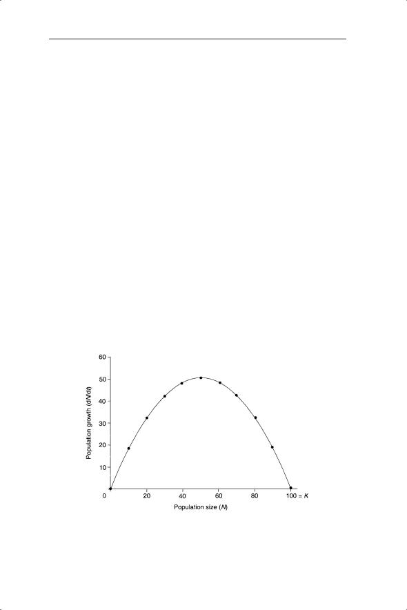
Assume that population growth is continuous and described by the logistic equation. Although in many cases the logistic equation is too simple a description of population change (see discussion in Chapter 5), it provides a useful entry point to understanding the dynamic possibilities of harvesting. We begin by plotting the rate of population growth, dN/dt, against population size, Nt (Fig. 6.13).
You should note that the curve in Fig. 6.13 is a parabola, which is the shape generated by a quadratic equation (recall that the right-hand side of the logistic equation in expanded form is rNt − rNt2/K). All population sizes which yield values of dN/dt > 0 can, in theory, be subject to harvesting. This means that a fraction of any growing population should be able to be harvested without causing the population to become extinct. The maximum sustainable yield occurs where the maximum value of dN/dt occurs; that is, when the population is growing most rapidly. This result is generally true for all population growth curves (see the discussion in May & Watts 1992).
Fig. 6.13 Population growth dN/dt described by the logistic equation plotted against population size (N). K is the carrying capacity.

MODELLING INTERACTIONS |
117 |
To determine the population density corresponding to the maximum sustainable yield we note that the maximum occurs when the gradient of the curve equals 0:
d(dN dt)dN = 0 |
(6.16) |
We will drop the subscript t to make the equations easier to read (N will still mean the population density at time t). For the logistic curve in Fig. 6.13 the derivative of the expression rN − rN2/K with respect to N is r − 2rN/K. Therefore
r(1 − 2(N K )) = 0
The solution to this equation is either r = 0 (a trivial solution) or (1 − 2(N/K)) = 0. Rearranging the latter yields the solution that N = K/2. So the population is growing at its fastest when it is half its maximum density. This agrees with the shape of the logistic curve where the point of inflexion (the maximum gradient) was at K/2 (Figs 5.11 and 6.13).
To find the maximum value of dN/dt we need to substitute the size at which the maximum occurs (K/2) for N in the logistic equation dN/ dt = rN(1 − N/K). This gives dN/dt = rK/4. This method of finding the maximum value is useful if the function for population growth is more complex than the logistic equation.
To develop these ideas let us assume a general form of population growth equation dN/dt = f(N) which describes the rate of change in population size as some function (f) of population size. If this function f(N) has a maximum value or values of dN/dt over a certain range of values of N then differentiation can be used to find the maximum value. You should note that the criterion of d(dN/dt)dN = 0 (equation 6.16) is not sufficient to identify a maximum value. It might equally identify a minimum value or a point of inflexion. A harvesting function can be incorporated into the general population growth equation (Beddington 1979):
dN dt = f (N ) − h(N ) |
(6.17) |
where h(N) gives the reduction in dN/dt at a particular value of N due to harvesting. The population change and harvesting functions of the generalized form of equation 6.17 can be combined on one graph as they are both functions of N (Figs 6.14 and 6.15). We will now consider several harvesting possibilities with a logistic growth curve.
If h(N) is constant and therefore independent of N, harvesting is represented by a horizontal line on the graph. We know that sustainable harvesting can only occur when dN/dt > 0; when f(N) > h(N) in equation 6.17. The area on the graph when this condition is met is shaded in Fig. 6.14 and lies between N = 20 and N = 80. What happens to the population at different population sizes? For example, consider a population of size 70. Here f(N) > h(N) and therefore population size increases (dN/dt > 0, equation 6.17).

118 CHAPTER 6
Fig. 6.14 Constant harvesting h(N) and logistic population growth f(N) plotted against N (equation 6.17). The shaded area shows where f(N) > h(N). Where the two lines (functions) intersect the rate of population change is 0.
Fig. 6.15 Linear increase in harvesting (h(N)) and logistic population growth (f(N)) plotted against population size (N).
In other words, from population size 70 we move to the right on the graph. Conversely, for a population of size 90, f(N) < h(N) and so dN/dt < 0 and the population size decreases.
By this reasoning it can be seen where h(N) = f(N) at N = 80 (and therefore dN/dt = 0) there is a locally stable equilibrium point. A population which receives a small displacement away from that equilibrium point will tend to return to it. What then of the other point at which dN/dt = 0, at N = 20? If

MODELLING INTERACTIONS |
119 |
N < 20 then f(N) is less than h(N) and therefore dN/dt < 0. So, the population will continue to decrease if reduced below 20 until it reaches N = 0, which is local extinction (N = 0 is effectively a third equilibrium point, which is locally stable). If the population size is increased above N = 20 then f(N) > h(N) and therefore the population size will continue to increase until it reaches the stable equilibrium point at N = 80.
Even the very simple scenario of constant harvesting combined with logistic growth provides the dynamic possibilities of extinction (below N = 20) and local stability (at N = 80). A second possibility for the harvesting function is that it increases linearly with prey population size (Fig. 6.15), so that the more fish there are, the more people go fishing. Again, N = 80 is seen as a stable equilibrium. In both this and the previous example, if the prey population is pushed beyond K (100) then it is predicted from the model that it will return towards K, but it will not stay there as h(N) is still greater than f(N) and therefore it continues to return to 80.
6.5.2 Structured population models
We begin by considering an unstructured population in discrete time in which the population dynamics are described by λ, the finite rate of population change, which is equivalent to the dominant eigenvalue of the population projection matrix for a structured population. We know that a population with λ < 1 will decline in numbers, so if a harvesting policy is to be sustainable it should not decrease the value of λ below 1. It is therefore possible to arrive at a simple definition of the maximum amount of a population which can be harvested. For example, if λ = 2, the maximum amount which can be removed is that which keeps λ = 1:
Fraction harvested = (λ −1) λ = 1 2
If λ = 3, the maximum fraction of the population which could be harvested is 2/3. This assumes that λ is constant from year to year and that a constant fraction is removed in each time period.
Now consider the implications of age, size or stage structure. To explore the effect of population structure on harvesting consider the two-stage model of biennial plants used previously (equations 4.9 and 4.10):
R |
|
0 |
|
= |
|
F |
s1,2 |
|
vt +1
fs0,1 R 0 F
M vt
The characteristic equation was λ2 = fs0,1s1,2 (equation 4.17). We know that the maximum fraction which can be harvested is given by (λ − 1)/λ, so it becomes of interest to see how manipulation of f, s0,1 and s1,2 affects (λ − 1)/λ.

120 CHAPTER 6
Assume that a fraction m1 of flowering plants is harvested prior to setting seed and therefore the fraction of surviving plants is represented by the fraction (1 − m1). Note that removal of flowering plants after seed set for a monocarpic species is not going to affect the population dynamics. This harvesting mortality can be incorporated into the model as follows:
R |
|
0 |
|
= |
|
F |
s1,2(1 − m1 ) |
|
fs0,1 R 0 F
vt +1 M with harvesting vt of F
In a similar way, we might imagine that a fraction m2 of rosette plants is harvested (of course, either m1 or m2 or both can have zero values). This can also be included in the model:
R |
|
0 |
fs0,1(1 − m2 ) R |
|
|
= |
|
0 |
|
F |
s1,2(1 − m1 ) |
F |
||
|
|
|
|
(6.18) |
vt +1 |
|
M with harvesting |
vt |
|
of F and R
We can now determine λ for the new model with the harvesting mortalities. The characteristic equation of the matrix equation 6.18 is:
λ2 = fs0,1(1 − m2 ) s1,2(1 − m1 ) |
(6.19) |
This is obviously similar to the characteristic equation without harvesting. Indeed, if we define λu as λ when the population is unharvested and λh as λ when the population is harvested, then we can derive a useful result from equation 6.19. Taking the square root of that equation:
λh = ± ( fs0,1s1,2 )r[(1 − m2 )(1 − m1 )]
As λu = ± ( fs0,1s1,2 )
λh = ±λu [(1 − m2 )(1 − m1 )]
Thus the value for λh is given by the original λ(λu) multiplied by the square root of (1 − m2)(1 − m1). Using matrices we can approach the problem from a slightly different angle to shed more light on the expression (1 − m2 )(1 − m1 ) .
Let us factorize the square matrix from equation 6.18:
|
0 |
fs0,1(1 − m2) |
|
|
|
0 |
|
s1,2(1 − m1) |
|
||
0 |
fs0,1 1 |
− m1 |
0 |
|
|
0 |
|
s1,2 |
0 |
1 − m2 |
|

MODELLING INTERACTIONS |
121 |
The left-hand matrix is the original transition matrix for the unharvested population and has an eigenvalue of λu. The right-hand matrix is composed of the two harvesting ‘survivals’ and can therefore be referred to as a harvesting matrix (Lefkovitch 1967). We could use this method for any structured population to explore the effects of harvesting of different ages, sizes or stages on population dynamics. Whereas matrix models can be valuable for analysis of the effects of harvesting and other management we need to be cautious as variations across time and space may alter λ and possibly reduce the maximum sustainable yield well below its theoretical value. For this reason, modellers have increasingly considered the role of stochasticity in harvesting models (Caswell 2000b). Sensitivity and elasticity analyses (Chapter 4) also help in interpretation of effects of harvesting.
Matrix models are now used routinely in investigating the effects of harvesting on structured populations. For example, Olmstead and Alvarez Buylla (1995) have explored the possibility of sustainable harvesting of two tropical palm species using matrix models. They calculated the population growth rates from stage-structured models and estimated the amount of adult trees which could be harvested per unit area. They concluded that only one species could be harvested as the λ of the other species was only 1.05. Similarly, a study of harvesting of Quercus in Mexico confirmed that removal of just 5% of adults could cause population decline (Alfonso-Corrado et al. 2007). Other studies have been applied to organisms as diverse as capybara (the world’s largest rodent; Federico & Canziani 2005) and red coral (Santangelo et al. 2007). Inevitably, such studies also have conservation applications as harvesting threatens the viability of a wide range of species.