

1gillman_m_an_introduction_to_mathematical_models_in_ecology
.pdfCHAPTER 7
Community models
7.1 Introduction to modelling of ecological communities
So far the emphasis has been on population dynamics of a single species or clade and two interacting species such as predators and prey or competitors. These pairwise interactions rarely occur in isolation. In this chapter we consider sets of interactions between an assemblage of species in a given locality, the dynamics of an ecological community. The evolutionary equivalent has been addressed briefly in terms of the diversity-dependent reductions in diversification rate. We will be asking similar questions of an ecological community as we did of a population; in particular we will be interested in the long-term stability of the community. In addition to the density of the population(s) a new variable arises in community dynamics: the diversity of the community. Although diversity is a major topic in its own right, for our purposes we simply need to know that the diversity of ecological has two components: species richness (the number of species) and the relative abundance of species; that is, their evenness (or not). It is these two components that are incorporated into diversity indices such as the Simpson and Shannon– Weiner indices.
The modelling of community dynamics has three related problems, which will be tackled in this chapter. First, there is a need to consider the full range of interactions between species (Chapter 6), described by all combinations of 0/+/− where 0 represents no interaction, + is a positive (beneficial) effect of species A on B and − is a detrimental effect of A on B (Fig. 7.1). The second problem is that we need to assign a strength – that is, a magnitude – to these interactions. The sign and magnitude of the interactions will be combined in a community matrix. Matrix methods will be used to investigate the stability and dynamics of communities. The final problem is the large number of species that may be present in a community. In response to this we will see how species can be objectively removed from the model to move towards the aim of the simplest realistic model.
These models of ecological communities will mostly assume a pool of species within a given area, each of which can change in abundance over time (including becoming locally extinct) but do not assume any immigration or possible replacement of species as seen during successional change.
122

COMMUNITY MODELS |
123 |
Fig. 7.1 Classification of interactions. Signs and magnitudes of aij are considered in section 7.2.
In addressing the structure and dynamics of large communities we should recognize that even the addition of one species to the two-species interactions of Chapter 6 produces important changes in the dynamics of the component species (Gilpin 1979, Guckenheimer & Holmes 1983, Schaffer 1985). An investigation of a food-chain model composed of just three species revealed that chaotic dynamics occurred within biologically feasible parameter values, whereas chaos was not possible in two species models (Hastings & Powell 1991).
7.2 Food-web structure and the community matrix
7.2.1 Introduction
Measures of complexity in ecological communities are often based on the composition of the community represented by the number and relative abundance of species. These measures, which include the myriad diversity indices, do not tell us very much about the functioning of communities and their properties, such as stability. To quantify functional aspects of the community and understand how they may respond to perturbations, we need to quantify the interactions between species. The potential complexity of such interactions in real ecological communities is illustrated by the food webs in Fig. 7.2.
The food web can be characterized by the number of component species and the average number of links between them. The latter is known as linkage density. This idea can be extrapolated to other interactions between species, such as mutualisms. A motivation of this work has been to understand how communities with different linkage densities might respond to environmental perturbations, for example pollution events. A naïve view of this suggests two alternative outcomes. A highly connected community (high linkage density) might be predicted to be more resistant to perturbations, for example because any one species will have many possible food sources. Alternatively we might imagine that a highly connected community will be less resistant because harmful effects on just a few species will potentially

124 |
CHAPTER 7 |
(a) |
|
No. of observations |
|
|
1–10 |
|
11–100 |
|
101–1000 |
|
>1000 |
|
Tetramesa brevicornis |
Festuca rubra |
|
|
Tetramesa brevicollis |
|
Ahtola atra |
Alopecurus pratensis |
Tetramesa angustipennis |
|
Tetramesa linearis |
Elymus repens |
Tetramesa hyalipennis |
|
|
|
Tetramesa cornuta |
Ammophila arenaria |
|
|
Tetramesa eximia |
Alamagrostis epigejos |
Tetramesa calamagrostidis |
|
Eurytoma sp. |
|
Eurytoma sp. |
|
Tetramesa petiolata |
Eschampsia cespitosa |
|
|
Tetramesa airae |
Dactylis glomerata |
Tetramesa longula |
Phalaris arundinacea |
Tetramesa longicomis |
|
Tetramesa albomaculata |
Phleum pratense |
|
|
Tetramesa phleicola |
Hypodium sylvaticum |
Tetramesa fulvicollis |
Bracon sp.1 Homoporus sp.2
Eurytoma sp. nr festucae2
Sycophila sp.1
Eurytoma sp.
Chlorocytus pulchripes Sycophila sp.3 Homoporus febriculosus3
Eurytoma tapio
Endromopoda sp.3
Sycophila sp.4
Pediobius sp.4 nr claridgei Eurytoma flavimana4
Eurytoma sp.4 nr apicalis Homoporus sp.4
Bracon erythorstictus
Eurytoma roseni
Chlorocytus agropyri5 Pediobius alaspharus5
Eurytoma sp. nr steffani Homoporus sp6 Homoporus fulviventris
Sycophila sp.6
Chlorocytus harmolitae Eurytoma danuvica6 Syntomaspis baudysi
Bracon sp.7
Endromopoda sp.
Homoporus luniger7
Eurytoma pollux
Eurytoma appendigaster Homoporus sp.
Pediobius sp. nr phralaridis8 Chlorocytus sp.8
Eurytoma castor8
Eurytoma erdoesi
Bracon sp.
Eurytoma phalaridis
Endromopoda sp.
Pediobius sp.
Pediobius claridgei
Bracon sp.
Eurytoma collaris
Pediobius festuscae
Pediobius eubius
Eupelmus atropurpureus
Endromopoda sp.
Macroneura vesicularis
Pediobius calamagrostidis
Chlorocytus deschampiae
Pediobius deschampiae
Endromopoda sp.
Mesopolopus graminum
Pediobius dactylicola
Chlorocytus phalaridis
Pediobius phalaridis
Chorocytus ulticonus
Pediobius |
Chorocytus |
planiventris |
formosus |
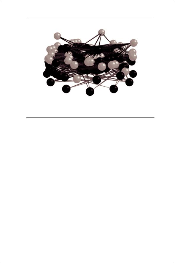
Fig. 7.2 Examples of food webs. (a) A grass–insect herbivore–parasitoid community used to demonstrate the effects of sampling effort (Martinez et al. 1999). (b) A diagrammatic view of a salt-marsh food web illustrating the complexity with inclusion of parasites (Lafferty et al. 2006, 2008). Parasites are light-coloured and free-living species are dark-coloured.
COMMUNITY MODELS |
125 |
(b)
Fig. 7.2 Continued
Table 7.1 A matrix of interaction coefficients for a hypothetical four-species community.
|
On species . . . |
Interaction coefficient |
|
||
|
|
|
|
|
|
|
|
A |
B |
C |
D |
|
|
|
|
|
|
Effect of species . . . |
A |
−1.0 |
−0.5 |
0 |
+1.0 |
|
B |
+0.5 |
−1.0 |
+0.5 |
0 |
|
C |
0 |
+0.5 |
−1.0 |
+0.8 |
|
D |
+1.0 |
0 |
−0.8 |
−1.0 |
|
|
|
|
|
|
cause major problems throughout the community. It is these types of questions that we will address in this chapter.
One way of describing the strength of interactions in a community is to construct a matrix of interaction coefficients. For example, a hypothetical four-species community can be represented as shown in Table 7.1. The representation can include both feeding and non-feeding interactions. For example, the effect of species A on species B is negative with a strength of 0.5. The intraspecific interactions (e.g. A on A) are all negative. Some of the interactions are symmetric, for example a positive effect of A on D and D on A, which is a fully mutualistic interaction. A value of 0 indicates no link between the species.
The analysis of ecological community stability is part of a wider debate about the stability or not of complex systems. Gardner and Ashby (1970) asked whether large systems (biological or otherwise) which were assembled
126 CHAPTER 7
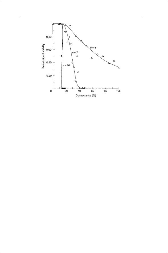
Fig. 7.3 The relationship between stability, connectance and component richness. A breakpoint or threshold of stability is observed at higher numbers of components. From Gardner and Ashby (1970).
at random would be stable. In their words, they were concerned with ‘an airport with 100 planes, slum areas with 104 persons or the human brain with 1010 neurons . . . [where] stability is of central importance’. Forty years on and these questions are no less pertinent; indeed, we may add an order of magnitude to some of these problems and present entirely new problems for solution; for example, global access to the Internet. Gardner and Ashby showed that for small numbers of components (n; e.g. neurons or species) stability declines with connectance between components (Fig. 7.3). As the number of components increases, the system moves rapidly to a breakpoint situation when a small change in connectance will result in a switch from stability to complete instability.
These results were developed by May (1972) in an ecological context. He concluded that increased numbers of species do not automatically imply community stability and in fact may produce just the opposite effect (see Jansen & Kokkoris 2003 and references therein for further debate on these results). Increased stability with complexity was promoted by Elton (1958), whose conclusions were partly based on detailed case studies of invasive species, such as the giant snail Achatina fulica into Hawaii and the red deer Cervus elaphus into New Zealand, which contributed to dramatic declines in the endemic species of those islands (see May 1984 and Pimm 1984 for a critique of Elton’s views). May also demonstrated that a species that interacts widely with many other species (high connectance) does so weakly (small interaction coefficient) and, conversely, those that interact strongly with

COMMUNITY MODELS |
127 |
others do so with a smaller number of species. He predicted that communities which are compartmentalized into blocks (effectively communities within communities) may be stable while the whole may not be. These ideas were explored further by Tregonning and Roberts (1979) who examined the stability of a randomly constructed model community in which the interaction coefficients were non-zero and the values chosen randomly. They began by running the model with 50 species, and used two methods of species elimination: a species was either chosen at random or the species with the most negative equilibrium value selected. Therefore, in the latter case they removed the most ecologically unrealistic species, as all species needed to have a positive equilibrium value. This process was continued until all species had a positive equilibrium value. This was defined by Tregonning and Roberts as the homeostatic system: one that was ecologically feasible and at equilibrium. Under selective removal the mean number of species comprising a homeostatic system was 25 and the largest 29. However, if elimination was random then the largest homeostatic system was 4 and the mean 3.3. Further understanding of these results requires a deeper insight into the nature of the community matrix used by May, Tregonning and Roberts and others. This is the subject of the next section.
7.2.2 Construction and stability of the community matrix
Levins (1968) first devised a matrix of Lotka–Volterra competition coefficients to describe community structure and predict community stability. This was a multi-species version of the two-species competition model (described earlier). This idea was developed by May (1972, 1973a) giving a general version of the matrix called the community matrix (sometimes referred to as the stability matrix) which expressed the effect of species j on species i near equilibrium. The community matrix makes some assumptions about the dynamics of its constituent species; in particular, it assumes that prey and competitors will be regulated so that in the absence of any interspecies interactions they will return to equilibrium. It is also assumed that predators decline exponentially in the absence of prey.
The community matrix allows insights into the stability of the community, with the dynamics of each species described by a nonlinear first-order differential equation. The aim is to create a matrix M of all interactions between the species in the community. It is assumed that species will be regulated so that, in the absence of any interspecies interactions, they will return to equilibrium. The following notation will be used:
αij the interaction coefficients between species i and j (expressed as the effect of species j on the growth rate of species i), including αii, the intraspecific interaction; the magnitude of α ranges from 1 to 0, which represents no interaction (the sign of α is considered below);

128 CHAPTER 7
Ni density or biomass of species i;
ri the intrinsic rate of change of species i; s the number of species.
A generalized Lotka–Volterra model following Roberts (1974) and Tregonning and Roberts (1979) and referred to by them as the multi-species quadratic model, is summarized for any number of species by:
|
|
|
s |
|
|
dNi |
dt = Ni |
ri + ∑ αij N j |
|
(7.1) |
|
|
|
|
i=1 |
|
|
|
|
|
|
|
|
where ri is positive for a producer (prey, competitor) and negative for a consumer (predator, pathogen) following the convention in Chapter 6. Therefore consumers decline exponentially in the absence of producers. Producers show density-dependent regulation as illustrated by the one-species version of equation 7.1:
dN1 dt = N1(r1 + α11N1 )
or
dN1 dt = r1N1 + α11N12 |
(7.2) |
This equation is equivalent to the logistic equation dN/dt = r1N1 − r1N12/K with α11 equal to −r1/K. Equation 7.2 shows why Tregonning and Roberts referred to the model as the (multi-species) quadratic model. In Chapter 5 it was shown that populations described by the logistic equation had a stable equilibrium of K. The equilibrium occurs at dN/dt = 0; therefore, for equation 7.2:
0 = rN1* + α11N1*2
where N1* is the equilibrium population size. Factorize the right-hand side to give N1*(r + α11N1*) and rearrange the non-trivial solution (r + α11N1*) = 0 to give:
N1* = −r α11
α11
As r must be positive for a single producer species, α needs to be negative to give a positive value of N1*. The sign of α is important and we will return to it later. (Note that the trivial solution is N* = 0.)
With two species, equation 7.1 gives:
dN1 |
dt = N1r1 + α11N1N1 + α12N2N1 |
(7.3) |
dN2 |
dt = N2r2 + α21N1N2 + α22N2N2 |
(7.4) |
We can compare the parameters α11, α12, α21 and α22 with the parameters in the competition and predator–prey equations in Chapter 6. In comparison with the competition equations, α11 = −r1/K1, α12 = −β12r1/K1, α21 = −β21r2/K2

COMMUNITY MODELS |
129 |
and α22 = −r2/K2. Generalizing for interactions between species i and j, αij = −βij ri/Ki and substituting αii for −ri/Ki, αij = βijαii; that is, the competition coefficient multiplied by the intraspecific interaction coefficient. Compared with the predator–prey equations 6.3 and 6.4 (assuming N1 is prey and N2 is predator): α11 = −r1/K1, α12 = −a, α22 = 0 and α21 = b. Also r2 will be negative and r1 will be positive.
We can therefore see how, with different values of r and αij, equation 7.1 can provide a generalized description of Lotka–Volterra dynamics covering interactions such as competition and predation.
The community matrix is then derived by considering the community at equilibrium. If we take the two-species example:
0 |
= N1*r1 + α11N1*N1* + α12N2*N1* |
(7.5) |
0 |
= N2*r2 + α21N1*N2* + α22N2*N2* |
(7.6) |
The species densities can be evaluated at equilibrium:
−r1 = α11N1* + α12N2*
−r2 = α21N1* + α22N2*
In matrix form this is |
|
|
|||
|
−r1 α11 |
α12 N1* |
(7.7) |
||
|
|
= |
|
|
|
|
−r2 |
α21 |
α22 N2* |
|
|
The values of N1* and N2* can be calculated using matrix algebra by finding the inverse of the matrix of coefficients and multiplying both sides to give:
|
−α22r1 + α12r2 |
|
|
|
N1* = |
|
|
(7.8) |
|
|
||||
|
α11α22 − α21α12 |
|
||
|
α21r1 − α11r2 |
|
|
|
N2* = |
|
|
|
(7.9) |
|
|
|||
|
α11α22 − α21α12 |
|
||
Matrix equation 7.7 can be generalized for any number of species as:
−r = AN*
where A is the square matrix of interaction coefficients and r and N* are column matrices of intrinsic rates of change and equilibrium densities respectively. Equilibrium values can then be found by matrix algebra as for equation 7.7 (equivalent to the solution of s simultaneous equations):
−rA−1 = N*
To determine the community matrix we need to linearize the population growth equation (7.1) at equilibrium. This is achieved with a Taylor expansion or series. A series is defined in mathematics as the sum of a sequence of numbers. We have seen how sequences may arise in ecological processes

130 CHAPTER 7
in Chapter 1 (Fibonacci sequence). Various functions such as ex or sin(x) can be expressed as a series. Using a Taylor series a function f(x + h) can be expressed as:
f (x + h) = f (x) + hf ′(x) + h2 2! f ′′(x) + h3
 3! f ′′′(x) + . . .
where x and h are both variables. f ′(x) means the derivative of the function evaluated at x whereas f ″ is the second derivative. If x represents the equilibrium density of a population which is described by a nonlinear function then when h is small (a perturbation from the equilibrium) the function near the equilibrium can be expressed according to the Taylor series as:
f (x + h) = f (x) + hf ′(x) |
(7.10) |
That is, ignoring terms with h2 and higher because h is relatively small. Equation 7.10 describes the linear tangent at equilibrium. In ecological communities we may be dealing with the abundances of many species, all of which have an equilibrium. In this case linearized dynamics are represented as partial derivatives in the Taylor series. Partial differentiation is a method of determining change in one variable while one or more other variables are held constant. Partial derivatives are indicated by ∂. Returning to equation 7.1 and writing it in general terms as:
dNi  dt = Fi(N )
the Taylor expansion around the equilibrium is:
dNi |
|
|
∂( |
dNi |
) |
|
|
|
|
dt |
|
|
|||||
k |
|
|
|
|
|
|
||
|
= Fi( N*) + ∑ j |
=1 nj |
|
|
|
|
+ secondand higher-order terms |
(7.11) |
dt |
∂N j |
|
||||||
|
|
|
|
|
|
|||
|
|
|
|
|
|
N * |
|
|
where nj is a small perturbation from equilibrium. Fi(N*) is 0 and secondand higher-order terms can be ignored. The partial derivatives ∂(dNi/dt)/∂Nj at equilibrium are αijNi*; that is, the interaction coefficient multiplied by the equilibrium population density of the ith species. You could check this for the two-species example. For example, to find ∂(dN1/dt)/∂N1 at N*:
∂(dN1 )
∂ dt = r1 + 2α11N1* + α12N2* (7.12)
N1
Substitute for N1* and N2* to give:
r1 |
+ |
2α11(−α22r1 + α12r2 ) |
+ |
α12(α21r1 − α11r2 ) |
|
α11α22 − α21α12 |
|||
|
|
α11α22 − α21α12 |
||
This reduces to:

|
COMMUNITY MODELS |
131 |
α11(−r1α22 + α12r2 ) |
|
|
|
α11α22 − α21α12 |
|
which is α11N1*. |
|
|
|
The full community matrix for the two-species example is: |
|
|
α11N1* α12N1* |
|
|
|
|
|
α21N2* α22N1* |
|
The stability of the community is found by determining the eigenvalue(s) of the community matrix. This tells us about the growth of a perturbation (nj) from equilibrium. If the sign of the largest eigenvalue of the community matrix is negative then the community is stable; that is, the perturbations reduce back in size towards the equilibrium. A positive value indicates growth of the perturbation away from the equilibrium. Therefore we can see why the community matrix is sometimes referred to as the stability matrix. The magnitude of the dominant eigenvalue determines the return time of the community (Pimm & Lawton 1977), which measures the time taken for a perturbation to decay to 1/e of its initial value.
To conclude this section we link up the graphical interpretation of stability of the logistic equation with the analytical method of the community matrix, following May (1973a) and Pimm (1982). Recall that there are two equilibria with the logistic equation (N* = 0 and N* = K). To examine the stability of those equilibria in Chapter 6 we used a graphical method to examine perturbations (displacements) from equilibrium and asked whether those displacements will become larger with time. If the perturbations do become larger then the equilibrium is locally unstable. From the community matrix analysis we expect that the stable equilibrium of the logistic model is given by a negative slope of dN/dt with respect to N at equilibrium; that is, the single ‘eigenvalue’ is negative. This is indeed the case (Fig. 7.4).
Fig. 7.4 Logistic curve showing unstable and stable equilibria. Note the gradient of the curves at N* = 0 and N* = K.