1gillman_m_an_introduction_to_mathematical_models_in_ecology

92 CHAPTER 5

their model provided a simple and useful description of the mechanisms underlying population growth (human or otherwise) and poetically invoked processes of density dependence and migration, as shown below.

In a new and thinly populated country the population already existing there, being impressed with the boundless opportunities, tends to reproduce freely, to urge friends to come from older countries and by the example of their wellbeing, actual or potential, to induce strangers to immigrate. As the population becomes more dense and passes into a phase where the still unutilized potentialities of subsistence, measured in terms of population, are measurably smaller than those which have already been utilized, all of these forces tending to increase the population will become reduced.

Pearl and Reed (1920), p. 287

The logistic curve has also been fitted to the growth of nonhuman populations, such as bacteria or yeast, with varying success. The best examples are cultures of algae, bacteria, insects and yeast (Fig. 5.13) where the simple assumptions of the logistic equation are most appropriate. The examples in Fig. 5.13 illustrate the sensitivity of r and K to genotype and environmental conditions.

Finally, given the models for the USA population it is of interest to consider what is happening to the world population (Fig. 5.14). Here, the raw data suggest that population increase has been approximately linear since the 1960s. This would suggest that the per-capita rate of growth is slowing. This is clear when we examine the ln (population size) (Fig. 5.15). Fitting a quadratic equation to the data since 1960 provides a very good fit (r2 = 0.9999). Using the quadratic function we can predict the increase and point of maximum population size assuming the same growth pattern since 1960. This is shown for the raw data (Fig. 5.16). The maximum value of 9.172 billion is predicted to occur in the year 2062. The addition of approximately 2.7 billion more people is clearly going to place profound stresses on the resources of the planet.

5.8 Density dependence in diversification rate

The importance of density dependence in population dynamics is reflected in studies of cladogenesis. In Chapters 2 and 3 we saw how clades might be expected to grow exponentially. Just as it is unrealistic to expect populations to continue to grow exponentially so it is unreasonable to expect clades to continue to diversify exponentially. As niche space becomes filled we may expect diversification rates to slow down. In this case the density is a density of species, rather than of individuals in the case of population dynamics. Tests of this hypothesis took on a new impetus in the 1990s with the advent of molecular phylogenies. In a seminal paper, Nee et al. (1992) demonstrated

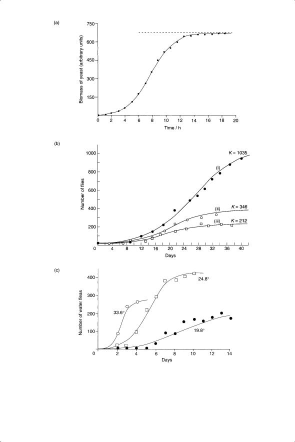
Fig. 5.13 Examples of applications of the logistic growth curve. (a) Growth of yeast populations in culture. From Allee et al. (1949) reprinted in Maynard Smith (1974).

(b) Growth of Drosophila melanogaster populations: (i) wild type, (ii) heterozygous or homozygous individuals for five recessive mutations including vestigial wing and (iii) wild type in half volume of (i). (c) Growth of Moina macrocarpa populations at three different temperatures. (b) and (c) reprinted from Hutchinson (1978).

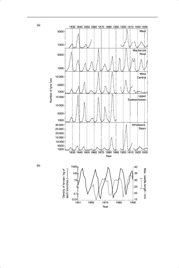
Fig. 6.1 Examples of cycling of abundance of predators and prey. (a) Cycles in the number of lynx (Lynx canadensis) fur returns of the Hudson’s Bay Company, from 1821 to 1934, grouped into five regions. Note the different scales (Elton and Nicholson 1942).

(b) Cycles of abundance of the monophagous larch bud-moth (Zeiraphera diniana) and the larch (variation in needle length). An 8–9 year cycle with a 10 000-fold change in larval density from peak to trough has occurred 16 times since 1850 in Switzerland (Baltensweiler 1993).

98 CHAPTER 6

(1926, 1928), who also derived equations to describe competition. The independence of their work is illustrated in their communications to the journal Nature from which the opening quotation to this chapter is taken (Lotka 1927). The premise of their predator–prey models, framed in continuous time, was that of:

. . . two associated species, of which one, finding sufficient food in its environment, would multiply indefinitely when left to itself, while the other would perish for lack of nourishment if left alone; but the second feeds upon the first, and so the two species can coexist together.

Volterra (1926)

Lotka and Volterra originally assumed that prey density (N) increased exponentially, quantified by r1, in the absence of predators (see also equation 2.10):

This was made more realistic by Volterra by assuming that change in prey density was described by the logistic equation that we met in Chapter 2; that is, the prey population would move towards an equilibrium of K in the absence of predation:

In the presence of predators the rate of change of prey population size with time, dN/dt, is assumed to be reduced in proportion a to the density of predators (P) multiplied by the density of prey (N):

As we are modelling a dynamic system in which the predator population density may also fluctuate, we need to develop an equation for dP/dt. Lotka and Volterra assumed that, in the absence of prey, the predator population size would decline exponentially, quantified by r2; that is, they assumed that the predator species specialized on one species of prey:

dP = −r2P dt

In the presence of prey, this decline would be counteracted by an increase in predator density, again in proportion to the density of predators (P) multiplied by the density of prey (N):

Equations 6.3 and 6.4 provide a system of two coupled first-order nonlinear differential equations. In section 6.2.2 we will consider a graphical technique for analysing the behaviour of coupled differential equations. This technique is very useful because systems of differential equations may arise in all the types of interaction considered in this chapter.

6.2.2 Phase plane analysis

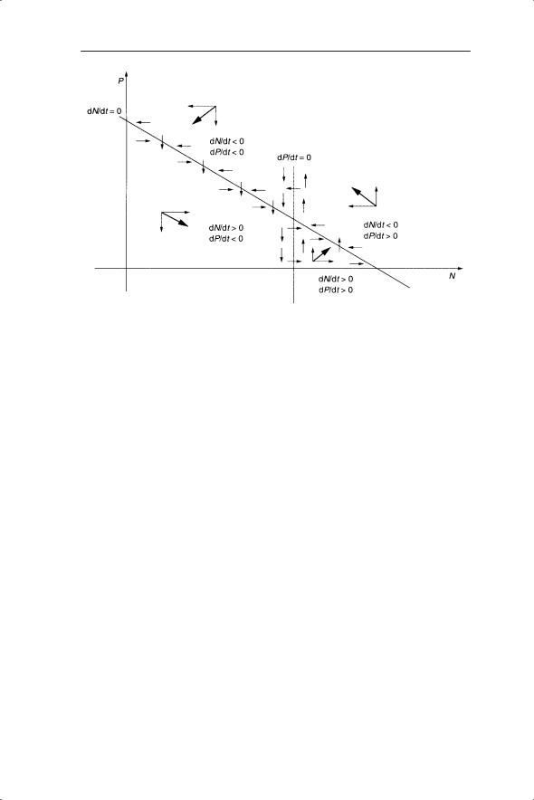
To understand the dynamics produced by the Lotka–Volterra equations we will examine their behaviour in a phase plane where the densities of predator and prey at time t are plotted and linked to their rate of change at those densities. This method of analysis was developed by Rosenzweig and MacArthur (1963). A phase plane can be used to describe change in coupled differential equations.

Begin at time 1 with a value of P1 for predators and N1 for prey (Fig. 6.2). To these densities we attach a vector showing the change in P and N from that point. The vector is a combination of two orthogonal vectors (vectors at right angles): one representing the value of dP/dt and one representing the value of dN/dt. The two vectors are added together to give the resultant vector (Fig. 6.2).

It is not necessary to know the precise direction of change from any given combination of N and P. Indeed, the beauty of phase-plane analysis is that the dynamics of the system can be understood by sketching some of the vectors based on the signs; that is, positive or negative values of dP/dt and dN/dt. Assume the following parameter values for equations 6.3 and 6.4:

Fig. 6.2 Prey (N) and predator (P) densities and representation of associated dynamics in the phase plane.

100 CHAPTER 6

r1 = 3 and r2 = 2 (prey > predator), a = 0.1, b = 0.3 and K = 10. Therefore dN/ dt = 3N − 3N2/10 − 0.1PN and dP/dt = −2P + 0.3PN.

Initially, we need to determine when dN/dt = 0 and dP/dt = 0 (known as zero-growth isoclines). First, dN/dt = 0 when 3N − 3N2/10 − 0.1PN = 0. This is equivalent to (3 − 3N/10 − 0.1P)N = 0 so that either N = 0 (the trivial solution in which prey are absent) or 3 − 3N/10 − 0.1P = 0. The latter can be rearranged to give P = 30 − 3N. This is a straight line equation that can be plotted on the phase plane (Fig. 6.3).

Similarly, dP/dt = 0 when −2P + 0.3PN = 0 or P(−2 + 0.3N) = 0. The solutions are either P = 0 (trivial solution) or −2 + 0.3N = 0; N = 2/0.3 = 6.667. This solution is plotted on the phase plane as a vertical line. The intersection of the two lines representing dN/dt = 0 and dP/dt = 0 is important, as this is where neither P nor N changes in density. The stability of this equilibrium point will be seen to be of great significance to the dynamics of the predator–prey system. The phase plane is divided up into four regions produced by the intersection of dN/dt = 0 and dP/dt = 0. Each region is characterized by a particular combination of positive or negative values of dN/dt and dP/dt (Fig. 6.4).

This is helpful as any point (N,P) in a given region will have a particular combination of vectors attached to it. Although the relative magnitudes of the vectors will depend on where the points are in the region, the overall direction of change in N and P (represented by the resultant vector) will always be the same. These directions are indicated as thicker arrows in Fig. 6.4.

Fig. 6.3 Lines representing no change in prey density (dN/dt = 0) and predator density (dP/dt = 0) on a phase plane.

Fig. 6.4 Overall direction of change in prey and predator densities in four regions of the phase plane.

So, to find the directions of the vectors in any region we need to determine whether dN/dt and/or dP/dt are positive or negative. For dP/dt, if N > 6.7 then −2 + 0.3N > 0 and dP/dt is positive (and vice versa). Therefore to the left of the dP/dt zero-growth isocline (at N = 6.7) all the change in P is negative (arrows point down in Fig. 6.4), whereas to the right the arrows point up. When dP/dt = 0 there is no change in P, so there can only be change in N, as indicated by the horizontal arrows. The direction of the horizontal arrows is only known when the regions of dN/dt greater or less than zero have been determined.

Now consider the two regions either side of dN/dt = 0. dN/dt < 0 occurs above the line of dN/dt = 0. You can check this by substituting values for N and P; for example P = 40 and N = 0 in the inequality 3 − 3N/10 − 0.1P < 0 gives 3 − 0 − 4 = −1. Therefore above the line of dN/dt = 0 the horizontal arrows point to the left and below the line they point to the right. When dN/dt = 0 there is no change in N so there can only be change in P, indicated by the vertical arrows with the direction determined by whether they are to the left or right of dP/dt = 0.

Now, for any point (N,P) in the phase plane we know the direction of change. Taking any starting point on the phase plane it is possible to look at the dynamics of N and P as a trajectory across the phase plane. With the above parameter values, starting at any point away from the equilibrium will send the population spiralling into the equilibrium point. An example of a trajectory under these conditions is given in Fig. 6.5.