

1gillman_m_an_introduction_to_mathematical_models_in_ecology
.pdf132 CHAPTER 7
7.3 Estimations of community stability and structure in the field
Seifert and Seifert (1976) provided one of the earliest field tests of the community matrix using insects in the water-filled bracts of Heliconia flowers in Central America (Fig. 7.5). The insects included larvae of chrysomelid beetles and syrphid flies, all of which were potential competitors.
Seifert and Seifert combined experimental manipulations with a multiple regression method which allowed them to estimate the magnitude and signs of the interaction coefficients from a generalized Lotka–Volterra model. This meant that statistical significance could be attached to each of the coefficients. The experiment involved emergent buds of Heliconia being enclosed in plastic bags to restrict immigration and oviposition. After a certain amount of growth, water was added and varying numbers of four species of insects were introduced. Following this the per-capita change in numbers with time was determined using a linearized version of equation 7.1, calculated as the change from initial density divided by the number of days over which the change took place. The initial densities of each species were used as the explanatory
Fig. 7.5 Stylized view of Heliconia wagneriana showing the dissected bract with common insect inhabitants. The species include Gillisius located on the dissected bract just above the water, Quichuana located at the base of the flower below Gillisius, Copestylum located just inside the flower and Beebeomyia located at the base of the seed. From Seifert and Seifert (1976).

COMMUNITY MODELS |
133 |
variables to calculate the partial regression coefficients of the per capita rates of change against all species; that is, this gave r and αij. (Note that the rates of change were not estimated from equilibrium as assumed by the community matrix.) A negative value of the regression coefficient indicated competition while a positive value indicated mutualism (the possibility of predation was ignored given the choice of insect species). From Table 7.2 we see that nine of the inter-specific interactions were not significant and therefore were set to zero. Of the significant ones, two were negative (competitors) and one was positive (mutualism).
The equilibrium densities estimated from the model by Ni* = A−1ri are shown in Table 7.3 compared with those observed in the field. The fact that there are two negative (unrealistic) densities for H. wagneriana suggests that the observed mean densities either are not equilibrium densities or are results of processes not dependent on species interactions, or that the model is inappropriate.
The eigenvalues of the community matrix were determined to examine the stability of the community. The four values were −0.0221, 0.052, −0.042 and −0.239. The positive eigenvalue indicated an unstable community. Seifert and Seifert’s conclusion was that H. wagneriana insect communities were indeed unstable and that migration, oviposition and local extinction processes may be important in structuring these communities. In other words it is probably not correct to model these communities in isolation. The effects of migration and local extinction are the subject of Chapter 8.
Table 7.2 Interaction matrix for Heliconia wagneriana. Non-significant coefficients are set to zero (Seifert & Seifert 1976).
|
Quichuana |
Gillisius |
Copestylum |
Beebeomyia |
|
|
|
|
|
Quichuana |
0.001 |
0 |
−0.018 |
0.027 |
Gillisius |
0 |
−0.003 |
0 |
0 |
Copestylum |
0 |
0 |
−0.005 |
0 |
Beebeomyia |
0 |
−0.005 |
0 |
−0.033 |
|
|
|
|
|
Table 7.3 Equilibrium densities predicted from the model compared with mean densities observed in the field (Seifert & Seifert 1976).
|
Mean densities in |
Estimated species |
|
unmanipulated examples |
equilibrium densities |
|
|
|
Quichuana |
51.00 |
−112 |
Gillisius |
7.56 |
−23.2 |
Copestylum |
8.78 |
4.09 |
Beebeomyia |
6.67 |
10.62 |
|
|
|

134 CHAPTER 7
Subsequent studies of the community matrix have covered a wide range of species. Wilson and Roxburgh (1992) provided examples of the application of the community matrix to plant species mixtures. They predicted that initially unstable six-species mixtures will, by selective deletion (following Tregonning & Roberts 1979), drop down to stable four-species mixtures. A study of the persistence of chironomid communities in the River Danube demonstrated differences in return times of perturbed communities at different sites (Schmid 1992). An analysis of local and global stability in six small mammal communities showed that all the community matrices were locally and globally stable, due to a reduction in connectance with increasing number of species (Hallett 1991).
The above examples show that it is possible to parameterize community matrix models using field data (with or without manipulations) and make testable predictions about stability, structure and return times after perturbation. Such predictions can be related to species richness and connectance. However, we need to be cautious as analysis of the community matrix is in the neighbourhood of an assumed equilibrium. For many applications we are likely to be interested in communities away from equilibrium or where non-equilibrium processes such as physical disturbance or pollution may be important. Local extinction and colonization processes may also mean that equilibrium has to be judged at larger spatial scales (Chapter 8).

CHAPTER 8
Spatial models
8.1 Spatial dynamics of host–parasitoid systems
In Chapter 6 we noted that Nicholson and Bailey had anticipated that spatial structure, in particular migration and local extinction, would lead to persistence in their model of host–parasitoid interactions. Comins et al. (1992) used the Nicholson–Bailey model to explore the possible outcomes of spatial dynamics. In this study it was assumed that the host and parasitoid were distributed among a square grid of square cells or patches of width n. These types of model systems, known collectively as cellular automata, have been widely used in both plant and animal studies to address a variety of issues including ecological stability and effects of invasive species (e.g. Crawley & May 1987, Silvertown et al. 1992, Colasanti & Grime 1993, Huang et al. 2008; see Wolfram 1984 for a mathematical overview).
Comins et al. (1992) had two phases of dynamics: reproduction/parasitism and dispersal. The former was modelled using the Nicholson–Bailey model. The latter had the following rules.
1A fraction of the hosts and parasitoids leave the patch (grid cell) and the remainder stay to reproduce in their patch.
2The fraction dispersing is equally divided between the eight neighbouring patches. There is only one movement per generation. Longer-range dispersal is excluded.
3There are reflective boundary conditions in which dispersing individuals are prevented from crossing the boundary and remain in the edge patch. Thus there is an explicit edge effect in this model, in contrast to some other cellular automata models.
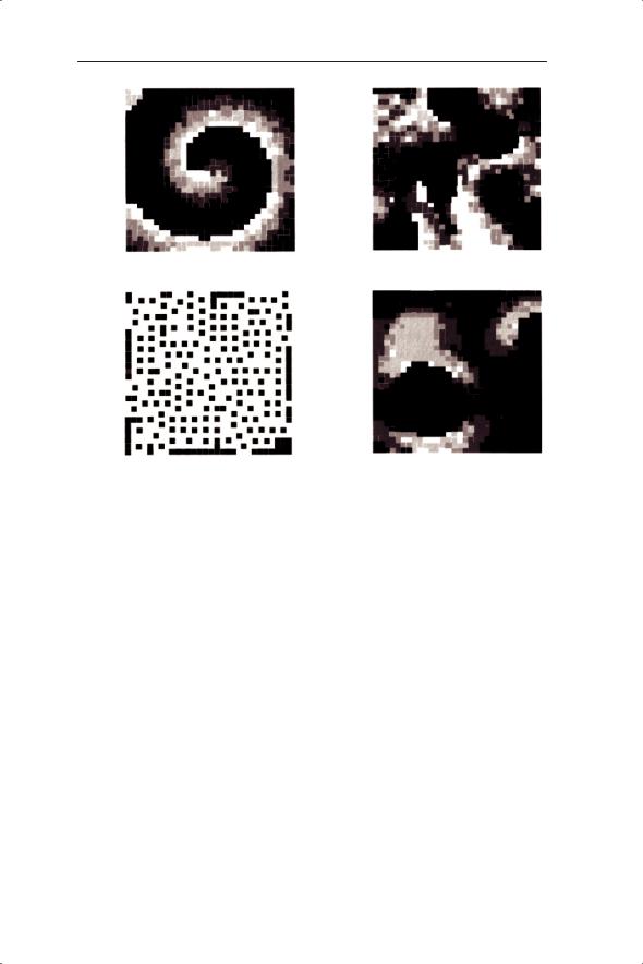
In small arenas of less than 10 cells by 10 cells extinction of host and parasitoid occurred within a few hundred generations of the simulations, underlining the inherent instability of the Nicholson–Bailey model. However, when the arena size was increased to between 15 and 30 patches, three general types of spatial dynamics were found which Comins et al. described as spirals, spatial chaos and crystal lattices (Fig. 8.1a). The key feature of the three dynamic types is that they permit long-term persistence of the host and parasitoid within a relatively narrow range of population densities (Fig. 8.1b), as
135
136 CHAPTER 8
Fig. 8.1 (a) Spatial dynamics of model host and parasitoid. Population density at one point in time from simulations after many generations of the dispersal model of Comins et al. (1992) using an arena width of 30 cells and with Nicholson–Bailey local dynamics. Different levels of shading represent different densities of hosts and parasitoids. Black squares represent empty patches. (i) Spirals, (ii) spatial chaos, (iii) crystalline structures. Case (iv) is a similar diagram obtained with Lotka–Volterra local dynamics which exhibits highly variable spirals. (b) Phase plane showing changes of host and parasitoid over time with the same corresponding parameters as in ai, aii and aiii.

SPATIAL MODELS |
137 |
did the incorporation of host density dependence or aggregation of parasitoids. Similar results were also found with the oscillatory unstable discrete version of the Lotka–Volterra model (Fig. 8.1a, panel iv). Other studies have explored the role of spatial dynamics of predators and prey as a contribution to the stability of their temporal dynamics. For example, McCauley et al. (1993) used an individual-based model to determine the relative importance of predator and prey mobility on stability.
In conclusion, a spatially explicit model can produce long-term population persistence in contrast to an unstable local population model. Mark–release– recapture data collected in the field are shedding light on the shortand long-distance dispersal capabilities of hosts and parasitoids. Jones et al. (1996), in a study of the movements of a tephritid fly (which feeds on thistle seed heads) and its parasitoids showed frequent movements across a patch of thistles of about 50 m × 50 m. The parasitoids moved further than the hosts within the patch. Longer-distance dispersal in similar organisms has been demonstrated by Dempster et al. (1995) using rubidium and other chloride salts in plants to mark herbivores and parasitoids. This work demonstrated that distances of up to 800 m are not a barrier to colonization.
In the next section we develop the theme of spatial models, focusing on analytical techniques rather than on the results of cellular automata simulations.
8.2 Metapopulation models
8.2.1 Introduction to the metapopulation concept
A metapopulation is defined as a set of local populations linked by dispersal. This could be described and modelled by cellular automata but we will focus on results arising from analytical considerations. In the original model of Levins (1969, 1970) it was assumed that all local populations were of equal size and that a local population could either become extinct or reach carrying capacity instantaneously following colonization. Therefore only two states of local population were envisaged: full (carrying capacity) or empty (extinct).
In reality, the definition of a local population, and therefore a metapopulation, is very difficult. Hanski and Gilpin (1991) defined a local population as a ‘set of individuals [of the same species] which all interact with each other with a high probability’. But how high is that probability? Furthermore, ‘local’ may be different for different interactions. For example, two plants may show intraspecific competition over a scale of a few centimetres but be reproductively linked by pollination over hundreds of metres. It is also very difficult to say over what distance colonization of new areas, and therefore the ‘birth’ of new local populations, may occur. Typically the frequency of movements of propagules such as seeds over short distances is known, but

138 CHAPTER 8
longer-distance movement is poorly known, partly because it may be a rare event and partly because it is difficult to record. This excludes species which show seasonal and predictable long-distance migration.
Even when local populations can be identified, the pure Levins model of local populations with equal carrying capacity is unusual. More realistically, it is reasonable to envisage a spectrum of possibilities from mainland/island or core/satellite to pure Levins populations (Fig. 8.2). These and other possi-
(a) |
(b) |
(c)
(d)
(e)
Fig. 8.2 Various types of spatial distribution of populations. Closed ovals represent occupied habitat patches and open ovals represent vacant habitat patches. Dashed lines indicate the boundaries of populations. Arrows indicate migration and colonization.
(a) Levins metapopulation. (b) Core/satellite metapopulation (Boorman & Levitt 1973).
(c) Patchy population. (d) Non-equilibrium metapopulation (differs from (a) in that there is no recolonization). (e) An intermediate case that combines (b) and (c) (Harrison 1991).

SPATIAL MODELS |
139 |
bilities have been discussed by Harrison (1991), who considered the rarity of true Levins metapopulations in the field, and by Hanski and Gyllenberg (1993), who showed how to model both mainland/island and pure Levins with related equations. Hanski (1999) provides an overview of the whole subject.
Various processes will promote something close to a metapopulation structure in the field or at least create conditions under which local extinction and colonization are integral features of the population dynamics:
•gap creation or other disturbance generating new recruitment habitat (includes habitat fragmentation);
•a mosaic of successional habitats where, for example, an annual plant must move from one transient early successional habitat to another (may be a function of the previous feature);
•sedentary and localized resources such as plants, dung or decaying logs, all of which may be colonized by various insects, fungi and other organisms. The resources may have a short colonization period allowing a maximum of one or a few generations of the attacking organism, thereby necessitating dispersal to other similar resources.
8.2.2 The metapopulation model of Levins
Despite the problems of finding Levins metapopulations in the field it is instructive to consider its dynamics before proceeding to more complex models. Levins (1969, 1970) was interested in the number of islands or island-like habitats occupied by a species. Later Levins and Culver (1971) modified the model to investigate the effect of competition on migration and extinction rates. Levins began by considering the number of local populations (N), the total number of sites (T), an extinction rate (e) and a migration rate (m′). The rate of change of N with time (t) could then be expressed as a differential equation:
dN dt = m′N(T − N ) − eN
This equation was simplified by using p = N/T where p represents the fraction of habitat patches occupied by a species and replacing m′T by m. The rate of change in the fraction of habitat patches occupied by a species, dp/dt – that is, the rate of change in the proportion of local populations (p) at a given time – was now described by:
dp dt = mp(1 − p) − ep |
(8.1) |
where m defines the colonization rate of local populations and e the extinction rate of local populations. Therefore ep represents loss (or extinction) of local populations from metapopulations. The birth rate of local populations is represented by mp(1 − p). The reason why p is multiplied by 1 − p can be

140 CHAPTER 8
conceptualized as a local neighbourhood problem. If there is one occupied patch surrounded by eight empty patches then the probability of colonization of any one empty patch is likely to be less than if there was one empty patch surrounded by eight occupied patches. Thus in determining the colonization probability the density of occupied patches and unoccupied patches needs to be combined, for example by multiplying them. In reality, the colonization (m) and extinction (e) parameters are likely to be complex functions of a set of variables. For example, m involves finding a new site, which depends on propagule dispersal (in turn dependent on the taxon and habitat under scrutiny and perhaps wind or water current speed or abundance of animal dispersers), the spatial distribution of occupied and unoccupied sites, initial establishment of propagules and subsequent population growth.
Now let us consider the dynamics of the system described by equation 8.1. What are the conditions for metapopulation increase, no change or decline? No change in p is given by dp/dt = 0:
0 = mp(1 − p) − ep
which gives
p = 1 − e m
m
Increase in p will occur if dp/dt > 0 and therefore p < 1 − e/m. In considering these results we need to think about the original formulation of the metapopulation concept. If extinction and colonization rates (death and birth) are balanced (e = m) there should be no change in metapopulation size. Similarly, if the extinction rate (e) is greater than the colonization rate (m) then the metapopulation size should decrease (and vice versa). These requirements are only partly supported by the manipulation of equation 8.1. The problem is that when dp/dt = 0, if e = m we are left with the result that p = 1 − 1 = 0. Thus, when extinction balances colonization there are no local populations. If colonization is greater than extinction then e/m is less than 1 but greater than 0 and therefore 1 − e/m lies between 1 and 0. Therefore a steady value of p occurs when colonization exceeds extinction. Hanski (1991) considers various refinements and developments of the basic Levins model. Despite the drawbacks of equation 8.1 we will see in the next section how it can be used to explain limits to species range and how more complex models can give similar predictions.
8.2.3 The Carter and Prince model of geographic range
The plant metapopulation model of Carter and Prince (1981, 1988) linked the ideas of Levins with models of infectious disease to provide an explanation for the geographical range limits of plant species. In particular, they challenged the view that distribution was determined solely by correlation to climate variables; for example, that the northerly distribution limit of plant

SPATIAL MODELS |
141 |
species in Britain was determined by physiological intolerance of cold winters (see examples in Carter & Prince 1988). Carter and Prince used a differential equation to describe a strategic model of plant distribution:
dy dt = bxy − cy |
(8.2) |
where x is the number of susceptible sites (sites available to be colonized), y is the number of infective sites (occupied sites from which seed is produced and dispersed), b is the infection rate and c is the removal rate. b and c are essentially local population birth (colonization) and death (extinction) rates and therefore equivalent to m and e in the Levins equation (8.1). Similarly, x and y are related to 1 − p and p where p is the proportion of local populations which are occupied and potentially ‘infective’ and 1 − p is the proportion of vacant and therefore susceptible sites.
These comparisons show that any conclusions from the Carter and Prince model are relevant to metapopulations in general as defined by Levins. The important conclusion of Carter and Prince was that, along a climatic gradient, a very small change in, for example, temperature might tip the balance from metapopulation persistence to metapopulation extinction. In Carter and Prince’s words: ‘a climatic factor might lead to distribution limits that are abrupt relative to the gradient in the factor, even though the physiological responses elicited might appear too small to explain such limits.’ Thus climate and physiological factors are still important but their effects are amplified and made nonlinear by the threshold properties of equation 8.2.
The results of these simple models are supported by the conclusions from more complex models. For example, the model of Herben, Rydin and Soderstrom (1991) examined the dynamics of the moss Orthodontium lineare which occurs on temporary substrates such as rotting wood. The model addressed not only the metapopulation structure of the moss but also the fact that the species was spreading throughout western and central Europe. The model included deterministic increase on occupied logs with a carrying capacity and the assumptions that dispersal by spores was in proportion to local population size and that spore dispersal distance declined exponentially from an occupied log. The results of this model suggested, like the simpler models, that there is a threshold for metapopulation persistence. In this case the percentage of logs occupied was a nonlinear function of probability of local population establishment (pest; Fig. 8.3).
At a pest value of about 0.0002 the model predicted a sudden increase in the percentage of occupied sites. So here was a threshold value above which metapopulation persistence was likely to be high. If pest is a function of climate then this would produce exactly the type of sharp break in species range predicted by Carter and Prince. It seems that such thresholds may be generated in a variety of ways. Below we consider how changes in gap frequency in grassland can generate a threshold for plant population abundance and how diffusion processes can lead to thresholds.