

24 NARROWBAND DIRECTION OF ARRIVAL ESTIMATION FOR ANTENNA ARRAYS
Figure 3.7: Roots of a polynomial whose coefficients are elements of a vector in the noise subspace with SNR = 20 dB. Three signals are present corresponding to the three roots that lie on the unit circle.
3.2.3 The Root MUSIC Algorithm
The root MUSIC algorithm was proposed by Barabell [20] and is only applicable for uniform linear arrays. It has been shown in [20] that the root MUSIC algorithm provides improved resolution relative to the ordinary MUSIC method especially at low SNRs. The steering vector for an incoming signal can be written again as defined in (2.10) and (2.13), i.e.,
an(θ) = exp( j 2 nd sin(θ)) , n = 0, 1, 2,..., N − 1 , |
(3.7) |
where d is the spacing between the elements in wavelengths and θ is the angle of arrival. As was the case before, the MUSIC spectrum is defined as:

Nonadaptive Direction of Arrival Estimation 25
PMUSIC = |
1 |
|
= |
1 |
, |
(3.8) |
aH (θ)Qn QHn a(θ) |
|
aH (θ)Ca(θ) |
||||
where C is |
|
|
|
|
|
|
|
C = Q QH . |
|
|
|
(3.9) |
|
|
n n |
|
|
|
|
|
By writing out the denominator as a double summation, one obtains [15]:
PMUSIC−1 |
= |
NΣ−1 NΣ−1 exp(−j2 pd sin θ) Ckp exp( j2 kd sin θ) |
(3.10) |
||
|
|
k = 0 p = 0 |
|
|
|
PMUSIC−1 |
= |
Σ |
Cl exp(−j 2 ( p −k)d sin θ). |
(3.11) |
|
|
|
|
p−k = constant = l |
|
|
Cl is the sum of the lth diagonal of the matrix C. A polynomial D(z) can now be defined as follows:
D(z) = |
NΣ+ 1 |
Cl z −l . |
(3.12) |
|
l= − N + 1 |
|
|
The polynomial D(z) is equivalent to PMUSIC−1 evaluated on the unit circle. Because the MUSIC spectrum will have r peaks, PMUSIC−1 will have r valleys and hence D(z) will have r zeros on the unit circle. The rest of the zeros of D(z) will be away from the unit circle. It can be shown [15] that if z1 = be jψ
is a root of D(z), then
be jψ = e j l sin(θ) b = 1, |
(3.13) |
||
where |
|
||
θ = sin−1 ( |
ψi |
) , i = 1, 2, . . . , d. |
(3.14) |
l |
|||
In the absence of noise, D(z) will have roots that lie precisely on the unit circle, but with noise, the roots will only be close to the unit circle. The root MUSIC reduces estimation of the DOAs to finding the roots of a (2N + 1)th-order polynomial.
3.2.4 The Minimum Norm Method
The minimum norm method was proposed by Kumaresan and Tufts [18]. This method is applied to the DOA estimation problem in a manner similar to the MUSIC algorithm. The minimum norm

26 NARROWBAND DIRECTION OF ARRIVAL ESTIMATION FOR ANTENNA ARRAYS
vector is defined as the vector lying in the noise subspace whose first element is one having minimum norm [17]. This vector is given by:
┌ |
1 |
┐ |
|
g = │gˆ |
││. |
(3.15) |
|
└ |
|
┘ |
|
Once the minimum norm vector has been identified, the DOAs are given by the largest peaks of the following function [17]:
PMN (θ) = |
│ |
1┌ |
1 |
┐ |
. |
(3.16) |
|
|
│ |
|
|||
|
│aH (θ)└│gˆ |
│┘│ |
|
|||
The objective now is to determine the minimum norm vector g. Let Qs be the matrix whose col-
umns form a basis for the signal subspace. Qs can be partitioned as [17]: |
|
|
|
|
|
Qs = |
α* |
(3.17) |
. |
||
Qs |
|
|
Since the vector g lies in the noise subspace, it will be orthogonal to the signal subspace, Qs, so we have the following equation [17]:
1 |
││= 0. |
|
QHs │gˆ |
(3.18) |
|
└ |
┘ |
|
The above system of equations will be underdetermined, therefore we will use the minimum Frobenius norm [17] solution given by:
gˆ = −Qˉ s (Qˉ Hs Qˉ s(
From (3.18), we can write:
I = QsH Qs = αα* −
From this equation, we can write:
¯ H |
¯ |
−1 |
α = ( I − αα |
* |
) |
−1 |
I = (Qs |
Qs |
|
|
|||
|
|
( |
|
|
|
|
−1 α .
Q¯ sH Q¯ s .
α = α/ (1 −||α||2) .
(3.19)
(3.20)
(3.21)
Using (3.21), we can eliminate the calculation of the matrix inverse in (3.19). We can compute g based only on the orthonormal basis of the signal subspace as follows:
Nonadaptive Direction of Arrival Estimation 27
¯ |
− || α|| |
2 |
) . |
(3.22) |
gˆ = −Qsα/ (1 |
|
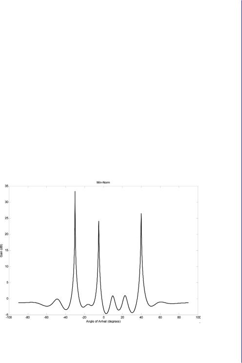
Once g has been computed, the Min-Norm function given above is evaluated and the angles of arrival are given by the r peaks (see Figure 3.8). The Min-Norm technique is generally considered to be a high-resolution method although it is still inferior to the MUSIC and estimation of signal parameters via rotational invariance techniques (ESPRIT) algorithms.
A simulation is performed with 10 sensors in a linear array tracking three signals, each with an SNR of 0 dB. The sensors are placed half a wavelength apart. Comparative performance results using the MUSIC algorithm, the Capon algorithm, the Min-Norm algorithm, and the classical beamformer are shown in Figure 3.9. It can be seen that the MUSIC algorithm and the Capon method identify the three signals and have no other spurious components. Of the two, the MUSIC algorithm is able to better represent the locations with more prominent peaks. The Min-Norm algorithm also identifies the signals similar to the MUSIC algorithm, but produces spurious peaks at other locations. The low-resolution classical beamformer identifies the three signals, but the locations are not represented by sharp peaks, due to spectral leakage. The classical beamformer also produces several spurious peaks.
Figure 3.8: The Min-Norm spectrum using a 10-element uniform linear array with three signals present each with an SNR of 0 dB. D = λ /2.