Добавил:

Upload Опубликованный материал нарушает ваши авторские права? Сообщите нам.

Вуз:

Национальный исследовательский университет «МИЭТ»

Предмет:

[НЕСОРТИРОВАННОЕ]

Файл:

Diss / 28.pdf

Скачиваний:

172

Добавлен:

27.03.2016

Размер:

7.05 Mб

Скачать

☆

<<< < Предыдущая 1 2 3 4 5 6 7 8 9 1011 / 1811 12 13 14 15 16 17 18 > Следующая >>>

40 NARROWBAND DIRECTION OF ARRIVAL ESTIMATION FOR ANTENNA ARRAYS

			│	1	cos					0				0 . . .
			┘
			│
			│				N
			│ 0		cos				cos		2			0 . . .
			│ 0		cos		N		cos		N			0 . . .
	µ		│				N				N
	µ		│
tan			│	0		0				0				0 . . .
tan	2		│	0		0				0				0 . . .
	2		│ .			.				.				. .	.
				.		.				.				.	.	.
			│ .			.				.				.		.
			│	0		0				0				0 . . .
			│	0		0				0				0 . . .
┘
│	0		sin					0		0 . . .				0
│	0		sin		N			0		0 . . .				0
│					N
│	0		sin			sin			2	0 . . .				0
│	0		sin		N	sin			N	0 . . .				0
│					N				N
= │	0			0				0		0 . . .				0
│ .				.				.		. .		.		.
	.			.				.		.		.	.
│ .				.				.		.			. .
│	0			0				0		0 . . .				0	sin
│	0			0				0		0 . . .				0	sin
┐	µ
tan	µ		Г1bN (µ) =					Г2bN (µ).

		2

0		0
0		0
0		0
.		.
.		.
.		.
0	cos	(N − 2)
0	cos	N
		N
	0

	(N − 2)	sin
	N	sin
	N

cos

(N − N

	0	│┐
		│
	0	│
	0	│
		│
	0	│ bN (µ)
	.	│
	.	│
	.	│
	(N − 1)	│
		│
	N	│
		┘
	│┐
	│
	│

│

││ bN(µ) ,

│

1)│

│┘

(3.78)

Now if r signals are present, then the transformed steering vectors are given by: bN(θ0), bN(θ1), …, bN(θr - 1); if a matrix B is formed using columns that are the transformed steering vectors, then this equation can be written as

Г1BΩ = Г2B, Ω = diag {tan	µ0	, tan	µ1	, . . . , tan	µr −1	} .	(3.79)
	2		2		2

The transformed steering vectors and the signal subspace of the transformed data vectors should span approximately the same subspace. Therefore, for some r × r matrix T, Es = BT and hence B = EsT–1. Substituting this equation in (3.79), we obtain

Г1EsT−1 Ω = Г2EsT−1, Г1EsΨ = Г2Es , with Ψ = T−1 ΩT .

(3.80)

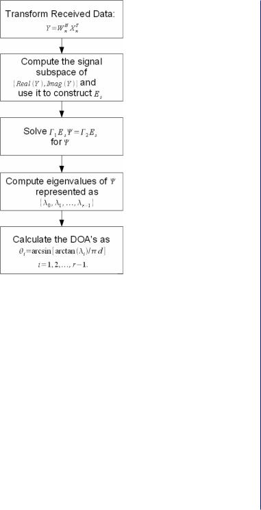
In Figure 3.13, we summarize the steps of the DFT beamspace ESPRIT [22].

3.2.11 The Multiple Invariance ESPRIT

It can be shown that the TLS ESPRIT algorithm is based on the following minimization problem [32]:

Nonadaptive Direction of Arrival Estimation 41

Figure 3.13: The DFT beamspace ESPRIT [22].

ˆ	10	] −	[BBΨ]││││,
{minB,Ψ} ││││[EEˆ				(3.81)

with B = AT and Ψ = T-1ΦT. We know that the actual signal subspace Es spans the same subspace as the columns of the steering matrix A; therefore, the two matrices could be related through a rotation matrix T, i.e., Es = AT. In the ESPRIT algorithm, a single invariance is exploited. A selection matrix is J = [J0T J1T ]T, where J0 is the (N - 1) × N matrix created by taking the first N – 1 rows of the N × N identity matrix and similarly, J1 is created by taking the last N – 1 rows of the same identity matrix. In the case of a uniform linear array, the following equation holds:

	[E1	]		¯
JE = JAT =	[E1	]	=	[A¯ Φ]	T.	(3.82)
JE = JAT =	E0		=	A	T.	(3.82)
s

Now suppose that the array has more than one identical subarray where the subarrays are displaced from the reference subarray by a vector that points in the same direction but has a different length.

42 NARROWBAND DIRECTION OF ARRIVAL ESTIMATION FOR ANTENNA ARRAYS

Let these vectors be ∆0, ∆1 , …, p – 1 and let J be a selection matrix for the subarrays with J =

[J0T J1T … J pT– 1]T.

	┘	E0	┐
	│	E0	│
	│	E1	│
JE = JAT │ .			│ =
s		.	│
	│ .		│
	│		│
	│Ep− 1		│
	┐		┘
	┐

┘	A	┐
│	A	│

│AΦ │

│ AΦδ2	│ T ,	(3.83)
.	│
│ .	│
│ .	│
│AΦδp −	1 │┘
┐

where δi = |∆i|/|∆1|. The multiple invariance ESPRIT (MI-ESPRIT) process is essentially based on a subspace fitting [30] formulation and can be posed as follows. First, a signal subspace estimate denoted Eˆ is computed for each subarray. Then, we determine the matrices A, Φ, and T that minimize the function V given below

┘

┐

┘

┐

││

││││

││

.δp −1

││

│

AΦ

│

AΦδ2

V =

│ .

│

−

│

(3.84)

│

│ .

┐ Ep − 1 ┘

┐ AΦ ┘

This minimization is nonlinear and in [32] it is solved by using Newton’s method. It is shown that the MI-ESPRIT algorithm outperforms ESPRIT, MUSIC, and root MUSIC, where performance is measured in terms of the root mean square error of the estimates.

3.2.12 Unitary ESPRIT for Planar Arrays

The unitary ESPRIT algorithm can be extended to two dimensions for use with a uniform rectangular array [31]. If an M × N rectangular array is used, the steering information will be contained in a matrix instead of a vector. This matrix is A(θx, θy ), where θx is the angle of arrival with respect to the x axis and θy is the angle with respect to the y axis. The matrix A(θx, θy ) can be transformed into a vector by stacking its columns thus forming a stacked steering vector a(θx, θy ). The (m, n) elements of the matrix A(θx, θy ) can be written as

A(θ, Ι )m,n = exp(−j 2πfcτm,n) ,			(3.85)
where
τn,m =	ndx sin(θx ) + mdy sin(θy)	,	(3.86)
τn,m =	c	,	(3.86)
	c

Nonadaptive Direction of Arrival Estimation 43

and c is the speed of the wave. Note that dx and dy are the spacing between columns and rows of the array in wavelengths, respectively. The matrix A(θx, θy ) can be written [31] as the outer product of two vectors of the form (3.40) as follows:

A(θx , θy) = aM (θx)aNT (θy) .

(3.87)

The matrix A(θx, θy ) has complex entries; they can be made real valued by premultiplying by QM and

postmultiplying by Q* . The real array manifold matrix then becomes

D(θx, θy) = QH aM (θx)aT		(θy)Q*	= dM (θx)dT	(θy) .	(3.88)
M	N	N	N

For the one-dimensional case, the invariance relation is given in (3.57). If this invariance relation is multiplied on both sides by dMT (θy ), the following result is obtained [31]

tan(u/2)K1D θx, θy = K2 D θx , θy .

(3.89)

D(θx, θy ) can be vectorized to create a vector d(θx, θy ) by stacking columns of D(θx, θy ). The above equation then becomes:

tan(u/2)Ku1d θx, θy =	Ku2d θx , θy ,	(3.90)
with	○
○	○
Ku1 = IM × K1, Ku2	= IM × K2 ,	(3.91)
where Hadamard products are used. Similarly, dT (θ ) satisfies
M y
tan(v/2)K3d(θy) = K4dN (θy) .		(3.92)
We then multiply the above equation on the right by dN(θx ) and we obtain:
tan(v/2)K3DT (θx, θy) =	K4DT (θx, θy) .	(3.93)
If we transpose both sides
tan(v/2)D(θx, θy)K3T = D(θx, θy)K4T .		(3.94)
The above equation can again be vectorized, i.e.,
tan(v/2)Kv1d(θx, θy) = Kv2d(θx, θy),		(3.95)

44 NARROWBAND DIRECTION OF ARRIVAL ESTIMATION FOR ANTENNA ARRAYS

and

= K

○

= K

○

(3.96)

Suppose that the incoming signals have angles of arrival: (θx1, θy1), (θx2, θy2), …, (θxd , θyd). A matrix

D can be formed from the vectors d(θx1, θy1), d(θx2, θy2), …, d(θxd , θyd ). The above equation can be written using matrix D as

Kv1DΩv = Kv2D,	(3.97)
where
Ωv = diag{tan d sin θy1 , . . . , tan d sin θyd } .	(3.98)
By the same argument,
Ku1DΩu = Ku2D,	(3.99)
and
Ωu = diag{tan ( d sin θx1), . . . , tan ( d sin θxd)}.	(3.100)

As was done for the uniform linear array, the data vector, x, obtained from the array may be transformed by QN and QM as follows:

y = QH XQ* ,							(3.101)
		N	M
or if y and x are to be vectorized:		○
y = Q	M	○	Q	M	x
y = Q	H	×	Q	H	x	.	(3.102)
	H			H		.	(3.102)

The data space is now spanned by {Re(y), Im(y)} and if Es is a basis for the signal subspace of the transformed data, then the columns of D and Es span the same space and can be related through an r × r matrix T, i.e.,

Es = DT, D = EsT−1.

(3.103)

Substituting for D in the invariance equations above, we get

Kv1EsT−1 Ωv = Kv2EsT−1 .

(3.104)

<<< < Предыдущая 1 2 3 4 5 6 7 8 9 1011 / 1811 12 13 14 15 16 17 18 > Следующая >>>

Соседние файлы в папке Diss

#
27.03.2016273.99 Кб682.pdf
#
27.03.2016398.45 Кб5723.pdf
#
27.03.20163.44 Mб5124.pdf
#
27.03.20162.49 Mб7825.pdf
#
27.03.20161.6 Mб5127.pdf
#
27.03.20167.05 Mб17228.pdf
#
27.03.20161.31 Mб523.pdf
#
27.03.2016838.41 Кб484.pdf
#
27.03.2016451.11 Кб425.pdf
#
27.03.201615.34 Mб486 - 753p.pdf
#
27.03.2016451.11 Кб406.pdf