


Nonadaptive Direction of Arrival Estimation 45
Let Ψv = T–1ΩvT. The DOAs can thus be computed by solving the above least squares problem and then finding the eigenvalues of the solution matrix, which contain the information [31] about the DOA.
3.2.13 Maximum Likelihood Methods
The maximum likelihood (ML) estimator performs better than the methods discussed previously but at the cost of increased computational complexity. This method can identify DOAs even for certain types of correlated signals. Assume that there are r signals arriving at angles, which are contained in the vector θ,
θ = [θ0 θ1 . . . |
θr −1 ] . |
(3.105) |
The matrix X is the data matrix whose ith column is xi. In this case [15], the joint probability density function of X is:
K −1 |
σ2I exp − σ12 |xi − A(θi)si |2 . |
|
f (X) = ∏i = 0 det1 |
(3.106) |
Neglecting the constant terms, the columns of A, or steering vectors, are functions of the elements of θ. The log likelihood function then becomes:
L = −Kd log σ2 − |
1 |
KΣ−1 |
|xi(l) − A(θ)si|2 . |
(3.107) |
2 |
||||
|
σ |
l = 0 |
|
|
Therefore, L must now be maximized with respect to the unknown parameters s and θ. This is equivalent to the following minimization problem:
minθk, s {iKΣ=−01 |xi − A(θi)si|2} . (3.108)
If θ is fixed and the function in (3.108) is minimized with respect to s, the least squares solution [15] can be written as:
si = (AH(θi ) A(θi))− 1AH(θ) xi. |
(3.109) |
Substituting the above least squares solution in the function in (3.108), we obtain:
minθk |
KΣ−1 |xi − A(θi) AH (θi)A(θi) −1 AH (θi)xi |2 |
} |
= minθk |
ΣL |xi − PA(θi)(θi)xi|2 |
} |
. (3.110) |
|
{i = 0 |
|
{i = 1 |
|
46 NARROWBAND DIRECTION OF ARRIVAL ESTIMATION FOR ANTENNA ARRAYS
The matrix P in equation (3.110) is a projector onto the space spanned by the columns of A. This is equivalent to maximizing the following log likelihood function:
K − 1 |
|
|
L(θ) = Σ |
|PA(θi ) xi|2. |
(3.111) |
i = 0 |
|
|
This function can be maximized by finding a set of steering vectors whose span closely approximates the span of the data vectors; note that the data vectors are the rows of X. This closeness will be measured by the magnitude of the projection of the rows of X onto the span of A. The choice of A that provides the largest magnitude is considered to be the closest [15].
3.2.13.1 The Alternating Projection Algorithm for ML DOA Estimation
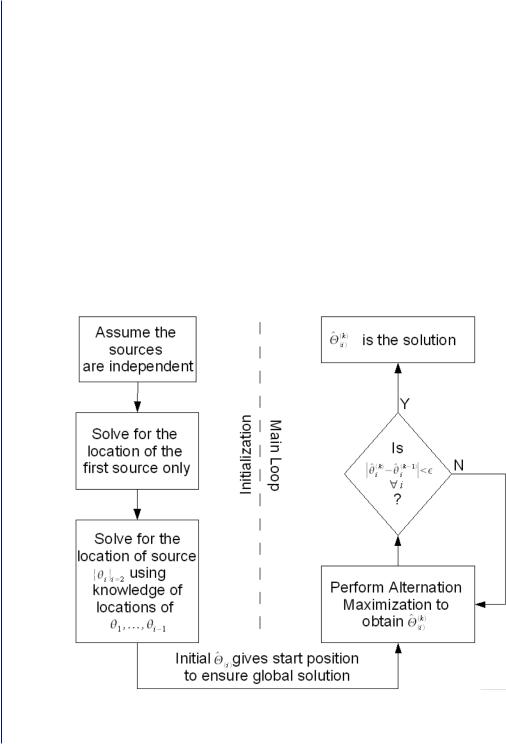
Ziskind and Wax [19] proposed an algorithm for maximizing the likelihood function in (3.107). The method is known as the Alternating Projection Algorithm (APA). The APA is shown in Figure 3.14 and summarized below:
Figure 3.14: The Alternating Projection Algorithm (APA) [19].

Nonadaptive Direction of Arrival Estimation 47
Step 1. Initialization: It is important to have a good initial guess of the matrix P so that the algorithm avoids convergence to a local minimum. This can be done by first finding a 1-D projection, P, that maximizes L. This projector will be constructed from a single vector from the array manifold. The angle corresponding to that vector will be the initial estimate of θ0. This vector is denoted a0(θ0). Now, we find the 2-D projector using a0(θ0) and a vector from the manifold that maximizes L. This vector will be called a0(θ1). This procedure is followed until P has been expanded into an r-dimensional projector. The initial estimates of the angles of arrival correspond to the steering vectors that are used to form the projection matrix P, i.e.,
[a0(θ0) a0(θ1) . . . a0(θr −1) ]. |
(3.112) |
Note that the superscript refers to the iteration number.
Step 2. Next, the steering vectors are held a0(θ1), a0(θ2), …, a0(θr − 1) fixed and we search for a new a0(θ0) that maximizes L. This new estimate of a0(θ0) replaces the old one and is denoted a1(θ0). We then proceed to hold a0(θ0), a0(θ2), …, a0(θr – 1) fixed and search for a new a0(θ1) that maximizes L. This new estimate of a0(θ1) will be denoted a1(θ1). We continue in this manner until a new estimate is obtained for each a1(θi). This constitutes one iteration.
Step 3. Repeat Step 2 until the variation in the vectors ak(θi) is below a certain tolerance factor.
• • • •

49
c h a p t e r 4
Adaptive Direction of
Arrival Estimation
The algorithms described in the previous chapters assumed that the data is stationary, which will be the case if the sources are not moving in space. When the sources are not stationary, then algorithms that continuously reestimate the direction of arrival (DOA) must be developed. For sources moving in space, the columns of the matrix A in (2.13) become time-varying and hence the span of the signal subspace will be changing with time. To track the signal subspace, a subspace tracking algorithm must be used. One way to develop an adaptive DOA algorithm is to concatenate a subspace tracker with a DOA algorithm. At each iteration, the subspace tracker passes an estimate of the signal or noise subspace to the DOA algorithm and it estimates the DOAs.
Adaptive versions of the estimation of signal parameters via rotational invariance tech niques (ESPRIT algorithm) that can efficiently update the DOA estimates with every iteration have been developed. In [6], it was shown that equation (3.31) can be solved adaptively. Another algorithm [13] is available that adaptively and efficiently computes the eigenvalues of (3.32). One of the benchmark algorithms for subspace tracking is Karasalo’s [28] subspace tracker.
Most subspace tracking algorithms are based on the N × N covariance matrix of the data and most algorithms use an exponentially weighted estimate of the covariance matrix in place of the estimator in (2.20), which is only useful when the signal sources are not moving in space. The equation for the exponentially weighted estimate at time n is
R |
xx |
(n) = αR |
(n − 1) + (1 |
− α)x |
n |
xH , |
(4.1) |
|
xx |
|
|
n |
|
where 0 < α < 1 is the forgetting factor. With a small forgetting factor, α, less emphasis is placed on past data and more emphasis is placed on the current data vector. A small value of α gives good tracking ability but poor steady-state accuracy, whereas a larger value of α gives slow tracking ability but provides good steady-state performance.

50 NARROWBAND DIRECTION OF ARRIVAL ESTIMATION FOR ANTENNA ARRAYS
Karasalo’s [28] subspace tracking algorithm uses the concept of deflation to reduce the dimension of the matrices involved from N × N to (r + 1) × (r + 2). Suppose that the eigendecomposition of the spatial correlation matrix Rxx(n) has the following structure:
|
H |
┌ |
┌ |
Ds(n) |
|
|
0 |
┐┌ |
H |
┐ |
|
Rxx(n) = Q(n)D(n)Q |
┐ |
|
2 |
│ |
Qs |
(n) |
(4.2) |
||||
|
(n) =│ Qs(n) Qn(n)││ |
0 |
σ |
(n)In |
││ |
H |
│, |
||||
|
|
└ |
┘ |
|
┘ |
Qn |
(n) |
|
|||
|
|
|
└ |
|
|
|
|
|
┘ |
|
|
|
|
|
|
|
|
|
|
└ |
|
|
|
where σr + 1(n) = σr + 2(n) = . . . = σN (n) = σ, Ds(n) = diag{σ1, σ2, …, σr}, and the columns of the matrix Q (n) = [Qs(n)Qn(n)] are the eigenvectors of Rxx(n). Because Rxx(n) is positive semidefinite,
the eigenvectors will form an orthogonal set and the eigenvalues will be real. The columns of Qs(n) form an orthonormal basis for the signal subspace and the columns of Qn(n), an orthonormal basis for the noise subspace. Ds(n) is a diagonal matrix that contains the signal eigenvalues of the matrix Rxx(n) and the noise eigenvalues are σ2(n). Therefore, all eigenvalues in the noise subspace are the same, which means that we have a spherical subspace. This means that any vector lying in that subspace, regardless of its orientation, will be an eigenvector with eigenvalue σ 2(n) and therefore the matrix Qn(n) can be rotated without affecting the above eigendecomposition of Rxx(n) as long as the columns of Qn(n) remain orthogonal to the signal subspace. Given this freedom, Qn(n) is chosen to be [w1(n)C(n)], where w1(n) is the normalized component of xn lying in the noise subspace and C(n) is a matrix whose columns form a basis for the subspace that is orthogonal to w1(n) and to the signal subspace. The data vector, xn, can be decomposed into these two components as follows:
xn = Q (n −1) zn + c1(n)w1(n) |
where |
wH (n)w1(n) = 1 |
and |
|
Q (n −1)w1(n) = 0 , |
|
(4.3) |
|||||||||||||||||
s |
|
|
|
|
|
|
|
|
1 |
|
|
|
|
s |
|
|
|
|
|
|
|
|
|
|
|
xn − |
Q (n −1)QH (n − 1)xn |
|
|
|
|
|
|
|
|
|
|
|
|
|
|
|
|
|
|
||||
|
|
|
|
√|| xn − Qs(n − 1)QHs (n −1)|| |
, |
|
|
|
|
|||||||||||||||
w1(n) = |
|
|
s |
s |
|
|
|
|
, c1(n) = |
|
|
|
(4.4) |
|||||||||||
|
|
|
|
|
|
|
|
|
|
|
||||||||||||||
√|| xn − Qs(n −1)QHs (n −1)|| |
|
|
|
|||||||||||||||||||||
|
|
|
|
|
|
|
|
|
|
|
|
|
|
|
|
|
||||||||
|
|
|
|
|
|
|
zn = QHs (n − 1)xn . |
|
|
|
|
|
|
|
|
|
|
|
|
(4.5) |
||||
|
|
|
|
┌ |
|
|
|
|
|
|
┐┌ |
|
|
|
|
|
|
|
|
┐ |
|
|
|
|
|
|
|
|
│ |
|
|
|
|
|
|
││ |
|
|
|
|
|
|
|
|
H |
|
|
|
|
|
Rxx(n) = (1 |
|
|
|
|
+ c1(n)w1 |
|
|
1)zn + c1(n)w1(n) |
│ |
|
|
|
|
||||||||||
|
− α)└Qs(n −1)zn |
(n) ┘└Qs(n − |
┘ |
|
|
|
|
|||||||||||||||||
The first term in the decomposition of xn |
in (4.3) lies in the signal subspace and the second term in |
|||||||||||||||||||||||
the noise subspace. Suppose the spatial covariance matrix Rxx(n) is updated using an exponentially |
||||||||||||||||||||||||
weighted estimate as given in (4.1), using (4.2)–(4.5) in (4.1), Rxx(n) can be written as: |
|
|
|
|||||||||||||||||||||
|
|
|
+ |
┌ |
|
|
|
|
┐┌ Ds(n −1) |
|
0 |
|
┐┌QH |
(n − |
1) |
┐ |
|
|
||||||
|
|
|
α│Q (n −1) Q |
n |
(n −1)││ |
0 |
σ2(n −1)In |
││ |
Q |
Hs |
(n − |
1) |
│ |
. |
(4.6) |
|||||||||
|
|
|
|
└ s |
|
|
|
┘ |
┘└ |
n |
┘ |
|||||||||||||
|
|
|
|
|
|
|
|
|
└ |
|
|
|
|
|
|
|
|
|
|
|
|
|||

Adaptive Direction of Arrival Estimation 51
The term on the right is the eigendecomposition of the spatial covariance matrix at time (n − 1). With some rearranging of the terms in the above equation and using Qn(n) = [w1(n)C(n)], (4.6) can be written as:
Rxx(n) = [Qs(n −1) w1(n)]│┌α1/2Ds1/2(n −1) |
||||
|
|
└ |
|
0 |
|
|
|
|
|
┌α1/2Ds1/2(n −1) |
|
0 |
||
× |
|
0 |
α1/2σ(n −1) |
|
│ |
(1 |
− α)1/2zH |
(1 |
− α)1/2c (n) |
└ |
|
n |
|
1 |
0(1 − α)1/2zn ┐│
α1/2σ (n − 1) (1 − α)1/2c1(n) ┘
┐ |
┐ |
(4.7) |
┌ |
|
|
││QHsw(1Hn(−n)1)│+ ασ2(n −1)C(n)CH (n) . |
|
|
└ |
┘ |
|
┘ |
|
|
The columns of the matrix term on the left lie in the subspace spanned by the columns of [Qs(n – 1)w1(n)]. The term on the right lies in the space spanned by the columns of C(n), which lies in the noise subspace. Therefore, the columns of the two matrix terms in (4.7) span two orthogonal subspaces. The columns of C(n) are eigenvectors of Rxx(n) that lie in the noise subspace. To compute the rest of the eigenvectors (the r signal eigenvectors and the remaining noise eigenvectors come from the first term), it is necessary to write the first term in (4.7) in terms of its eigendecomposition U(n)D(n)UH(n). This can be done by first computing the singular value decomposition (SVD) of the (r + 1) × (r + 2) matrix
L(n) = |
┌ |
α1/2Ds1/2(n −1) |
0 |
(1 −α)1/2zn |
┐ |
. |
|
│ |
0 |
α1/2σ(n −1) |
(1 −α)1/2c1(n)│ |
||||
|
|
||||||
|
└ |
|
|
|
┘ |
|
|
Suppose its SVD is V(n)S(n)YH(n), then the first term in (4.7) can be written as:
|
┌ |
H |
|
Rxx(n) = [Qs(n −1) w1(n) ]V(n)S(n)YH (n)Y(n)SH (n)VH (n) │Qs |
|||
|
└ |
w |
|
|
|
||
+ ασ2 (n −1)C(n)CH (n) |
|
|
|
┌ |
|
┐ |
|
= [Qs(n −1) w1(n) ]V(n)S(n)SH (n)VH (n)│QHws (Hn(−n)1) |
│ |
|
|
└ |
1 |
┘ |
|
+ ασ 2(n −1)C(n)CH (n)
=K(n)S(n)SH (n)KH (n) + σ2(n −1)C(n)CH (n)
= |
|
K(n) C(n) |
┌S(n)SH (n) |
0 |
┐┌KH (n) |
||
[ |
] │ |
0 |
ασ 2(n −1)IN − r −1 |
││CH (n) |
|||
|
|
||||||
|
|
|
└ |
|
|
┘└ |
|
┐
(n −1) │ H1 (n) ┘
┐
│.
┘
(4.8)
(4.9)

52 NARROWBAND DIRECTION OF ARRIVAL ESTIMATION FOR ANTENNA ARRAYS
The matrix Rxx(n) is now in its eigendecomposition form and it has been assumed that K(n) = [Qs(n – 1)w1(n)]V(n). Assume also that the SVD has been computed in such a way that the diagonal elements of the matrix, in the middle of the above product, are in descending order. Then the signal eigenvectors, or those corresponding to the largest eigenvalues of Rxx(n), are the first r columns of K(n) and the noise eigenvectors of Rxx(n) are the columns of C(n) and (r + 1)st column of K(n). If the (r + 1) x (r + 1) matrix V(n) is partitioned as follows:
┌ |
|
|
┐ |
|
V(n) = │ |
θH(n)** │, |
(4.10) |
||
└ |
f |
(n) |
┘ |
|
|
|
|
||
where the matrix θ(n) has dimensions r × r and the vector f H(n) has dimensions 1 × r, then the updated signal subspace can be written as
Q (n) = Q (n −1) |
θ(n) + w (n)f H (n) |
. |
(4.11) |
|
s |
s |
1 |
||
Table 4.1: Summary of Karasalo’s Subspace Tracking Algorithm [119, 121]
Initialization
for n = 1, 2, ....
zn = QHs (n − 1)xn |
|
|
|
|
|
|
|
||||||||
w1(n) = x(n) − Qs(n −1)z1(n) |
|
|
|
|
|
||||||||||
c (n) = wH |
|
(n)w (n) |
|
|
|
|
|
|
|
||||||
1 |
|
1 |
|
|
|
1 |
|
|
|
|
|
|
|
|
|
w1(n) = w1(n)/ √ |
|
|
|
|
|
|
|
|
|
||||||
c1(n) |
|
|
|
|
|
|
|
||||||||
┌ |
α1/2Ds1/2(n −1) |
|
|
0 |
|
(1 −α |
1/2)1/2zn |
┐ |
|||||||
L(n) = │ |
α |
1/2 |
|
│ |
|||||||||||
└ |
|
|
|
|
|
0 |
|
|
σ(n −1) |
(1 −α) c1(n) |
┘ |
||||
|
|
|
|
|
|
|
|
|
|
|
|
|
|
||
L(n) = V(n)S(n)YH(n). |
Perform SVD of L(n). |
|
|
||||||||||||
┌ |
θ(n)* ┐ |
|
|
|
|
|
|
|
|||||||
V(n) = │ |
f |
H |
|
*│ |
|
|
|
|
|
|
|
||||
└ |
|
|
(n) |
┘ |
|
|
|
|
|
|
|
||||
|
|
|
|
|
|
|
|
|
|
|
|
||||
Q (n) = Q (n −1)θ(n) + w1(n)f H (n) |
|
|
|
|
|||||||||||
s |
|
s |
|
|
|
|
|
|
|
|
|
|
|
|
|
|
|
|
1 |
|
|
|
|
N |
− r −1 |
(n − 1) |
|
|
|||
σ2(n) = ———σr2+1(n) + α ————σ2 |
|
|
|||||||||||||
|
N |
− |
r |
|
|
|
N − r |
|
|
|
|
||||
end(n)