

20 NARROWBAND DIRECTION OF ARRIVAL ESTIMATION FOR ANTENNA ARRAYS
with a half-wavelength spacing. Three signals with equal power are present and it is clear that the MVDR method (solid line) offers superior performance. In this simulation, the data vectors were generated using (2.12) and Rxx was computed using (2.20). Three signals were present, and (3.1) and (3.2) are plotted for angles between −90° and +90°.
3.2SUBSPACE METHODS FOR DOA ESTIMATION
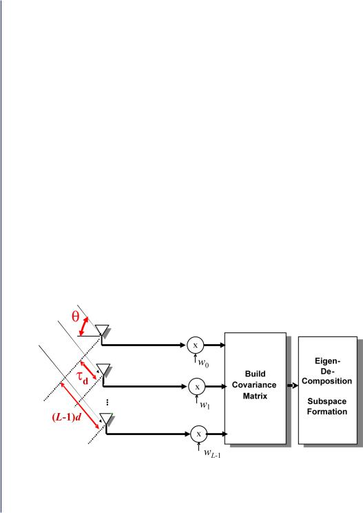
In this section, DOA estimators that make use of the signal subspace are described. These DOA estimators have high-resolution estimation capabilities. Signal subspace methods originated in spectral estimation [6] research where the autocorrelation (or autocovariance) of a signal plus noise model is estimated and then used to form a matrix whose eigenstructure gives rise to the signal and noise subspaces. The same technique can be used in array antenna DOA estimation by operating on the spatial covariance matrix as shown Figure 3.3.
3.2.1 Multiple Signal Classification Algorithm
It was shown in Chapter 2 that the steering vectors corresponding to the incoming signals lie in the signal subspace and are therefore orthogonal to the noise subspace. One way to estimate the DOAs is to search through the set of all possible steering vectors and find those that are orthogonal to the noise subspace. If a(θ) is the steering vector corresponding to one of the incoming signals, then
Figure 3.3: Eigendecomposition of antenna array signals. θ is the angle of arrival; D is the distance between two adjacent elements in meters; τ d is the time delay of arrival between two successive elements in seconds; and there are L elements in the array.
Nonadaptive Direction of Arrival Estimation 21
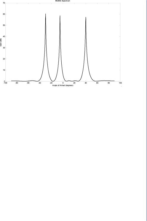
Figure 3.4: The MUSIC spectrum using a 10-element uniform linear array with three signals present each with an SNR of 0 dB. d = λ /2.
a(θ)HQn = 0. In practice, a(θ) will not be precisely orthogonal to the noise subspace due to errors in estimating Qn. However the function
PMUSIC(θ) = |
1 |
(3.4) |
|
aH (θ)Qn QnH a(θ) |
|||
|
|
will assume a very large value when θ is equal to the DOA of one of the signals. The above function is known as the multiple signal classification (MUSIC) “spectrum” (Figure 3.4). The MUSIC algorithm, proposed by Schmidt [11], first estimates a basis for the noise subspace, Qn, and then determines the r peaks in (3.4); the associated angles provide the DOA estimates.
The MUSIC algorithm has good performance and can be used with a variety of array geometries. The disadvantage of the MUSIC algorithm is that it is not able to identify DOAs of correlated signals and is computationally expensive because it involves a search over the function PMUSIC for the peaks. Spatial smoothing can be introduced to overcome this problem. In fact, spatial smoothing is essential in a multipath propagation environment. To perform spatial smoothing, the array must be divided up into smaller, possibly overlapping subarrays and the spatial covariance matrix of each subarray is averaged to form a single, spatially smoothed covariance matrix. The MUSIC algorithm is then applied on the spatially smoothed matrix.
The following simulation illustrates the effect of spatial smoothing as used with the MUSIC algorithm. Consider the typical array antenna scenario depicted in Figure 1.3 or for the planar
22 NARROWBAND DIRECTION OF ARRIVAL ESTIMATION FOR ANTENNA ARRAYS
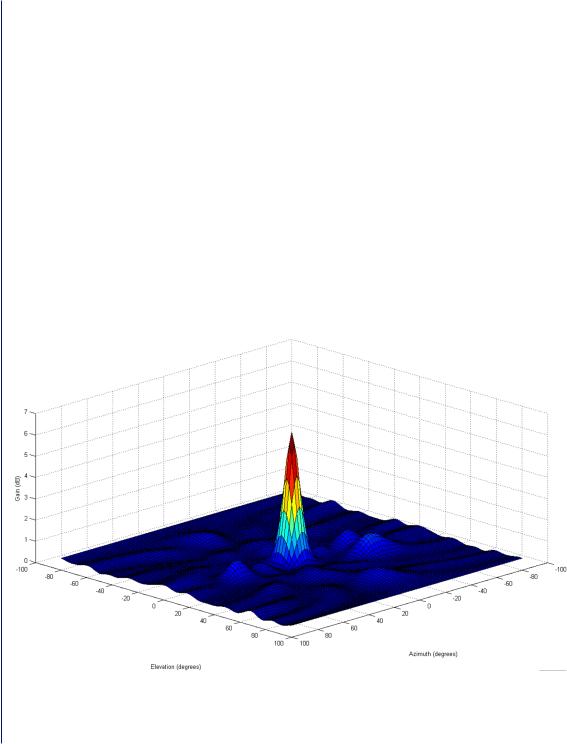
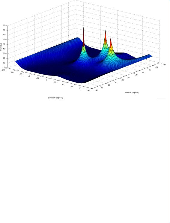
antenna array shown in Figure 1.4. A simulation where the receiving planar antenna array consists of 64 elements placed in an 8 × 8 grid is performed. Consider that three correlated signals arrive at the array from different directions due to multipath propagation. The direct line of sight signal arrives with a 0-dB SNR, whereas the two reflected signals arrive with −3 dB and −5 dB SNRs, respectively. Figure 3.5 shows the two-dimensional (2-D) MUSIC spectrum without spatial smoothing, which has a peak at the angle of arrival of the direct line of sight signal. The angles of arrival of the two reflected signals are not clear. In Figure 3.6, a simulation of the MUSIC algorithm with spatial smoothing is shown. In this case, the three signals are distinct.
3.2.2 Orthogonal Vector Methods
Consider a vector, u, orthogonal to the columns of the matrix A (i.e., uHA = 0), which implies that
u lies in the noise subspace, u = [u*, u*, …, u* ]T. Because the inner product of u with any of the |
|
0 1 |
N − 1 |
r columns of A is zero and the structure of the columns of A for the uniform linear array is known, the following expansion of the inner product can be written as
uH a(θi) = u0 + u1e− jωi + u2e− j 2ωi + · · · + uN −1e− j(N −1)ωi = 0 . |
(3.5) |
Figure 3.5: The MUSIC spectrum using an 8 × 8 element planar array with three signals present where no spatial smoothing is used; D = λ /2. Only one signal is detected.
Nonadaptive Direction of Arrival Estimation 23
Figure 3.6: The MUSIC spectrum using an 8 × 8 element planar array with three signals present where spatial smoothing is used. D = λ/2.
Define the polynomial u(z) as:
u(z) = u0 + u1z + u2z 2 + · · · + uN −1z N −1 |
(3.6) |
Equations (3.5) and (3.6) indicate that the polynomial u(z) evaluated at exp(–jωi ) is zero for i = 0, 1, …, r − 1. Therefore, the r of the roots of u(z) lie on the unit circle (i.e., they all have magnitude equal to 1). Because the angles, ωi, of these roots are functions of the DOAs (recall that ωi = 2 dsin(θi)), the roots of u(z) can be used to compute θi.
To summarize the orthogonal vector methods, any vector that lies in the noise subspace is first computed. Next, a polynomial is formed whose coefficients are the elements of that vector. The r roots of the polynomial that lie on the unit circle are computed and used to determine the DOAs. This method does not work well when the SNR is low but high-performance methods based on this idea are available. Figure 3.7 shows the roots of a polynomial for a uniform linear array with 10 elements. There are three signals and nine noise components, with an overall SNR of 20 dB. The orthogonal vector methods based on this idea include Pisarenko’s algorithm [29], the root MUSIC [20], and the Min-Norm [4] techniques, which are discussed next.