Adaptive Direction of Arrival Estimation  53

Next, the estimate of σ 2(n) is updated from the new eigendecomposition of Rxx(n) given in (4.9), where the diagonal elements of S(n) are σ 1(n) ,σ 2(n) , …, σr + 1(n) and have been placed in descending order. The N – r noise eigenvalues are σr2 + 1(n), ασ 2(n – 1), ασ 2(n – 1), …, ασ 2(n – 1), where ασ 2(n - 1) is listed N – r – 1 times. Taking an average of these values gives

Karasalo’s method is an SVD updating algorithm and is often used as a reference method for comparing other subspace tracking algorithms. Although it is a good reference method, Karasalo’s algorithm is not often used in certain practical applications because the computation of the (r + 1) × (r + 2) SVD at each iteration is itself an iterative process. Other similar algorithms exist that replace the (r + 1) × (r + 2) SVD with a more efficient adaptive method [27, 28].

4.1ADAPTIVE SIMULATION EXAMPLE

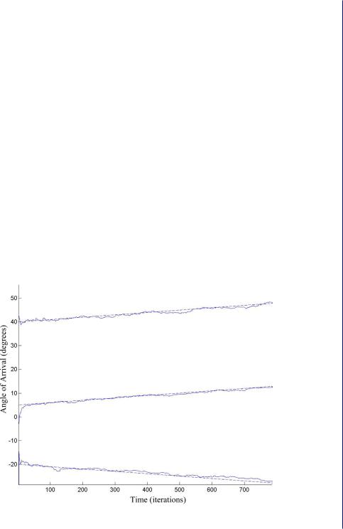
In this simulation, there are three signal sources moving in space with time. Their DOAs are changing by 0.01° per iteration. The subspace tracking algorithm in Table 4.1 is used to track the signal subspace. The DOAs are recomputed after each iteration using the estimate of the signal subspace, Qs, and the ESPRIT algorithm given in (3.31)–(3.33a). The dotted line in Figure 4.1 represents the true DOA and the solid line represents the estimate of the DOA by the adaptive algorithm.

Figure 4.1: Adaptive DOA simulation using Karasalo’s subspace tracker and the ESPRIT algorithm.